
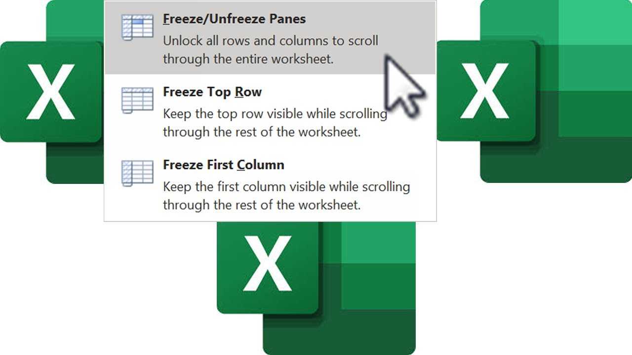
Freeze Panes with VBA
Using the Freeze Panes feature is easy when you’re working with a single sheet. But if you have many similar sheets on which you want to freeze the top row and first column it can be a tedious task!
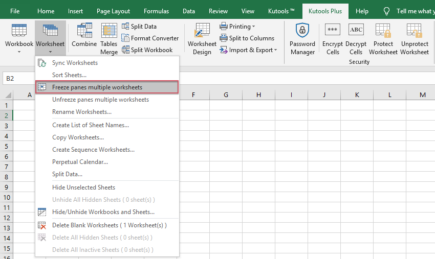
You would need to select each sheet, then select cell B2 within, then turn on the Freeze Panes feature. That could be a lot of clicks.
This is definitely a task that can be automated with the use of VBA!
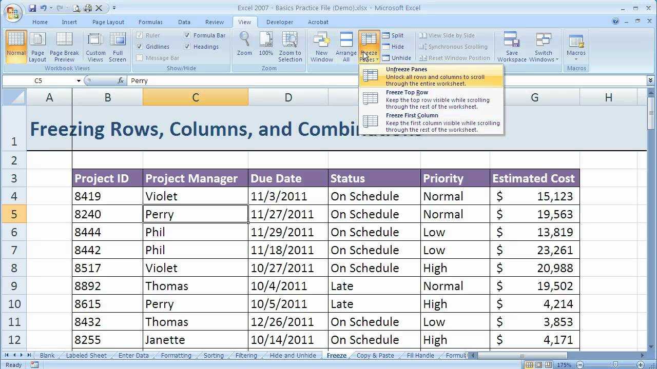
Go to the Developer tab and click on the Visual Basic option to open the visual basic editor. Go to the Insert menu in the editor and select the Module option.
Copy and paste the above code into the new module in the editor.
When you run this VBA code it will look through all the sheets in the workbook, then select cell B2 and turn on the Freeze Panes option.
This will make quick work of freezing the first row and first column across your entire workbook!
Freeze First Column
This feature could be used to freeze a particular column that you would need to refer while working on excel. In this option only the first column will freeze.
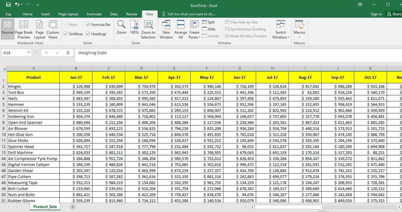
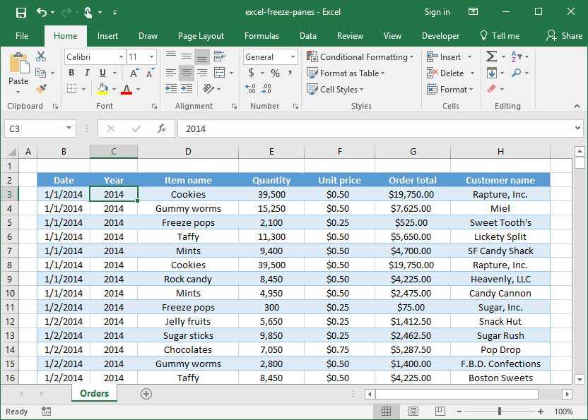
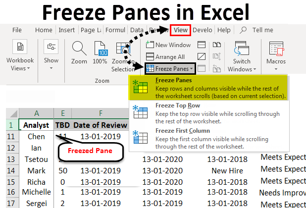
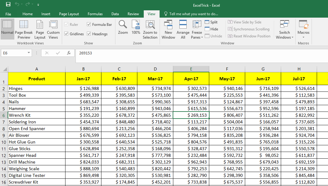
Open the sheet where in you want to freeze the column, as an example we would like to freeze the column A – Product
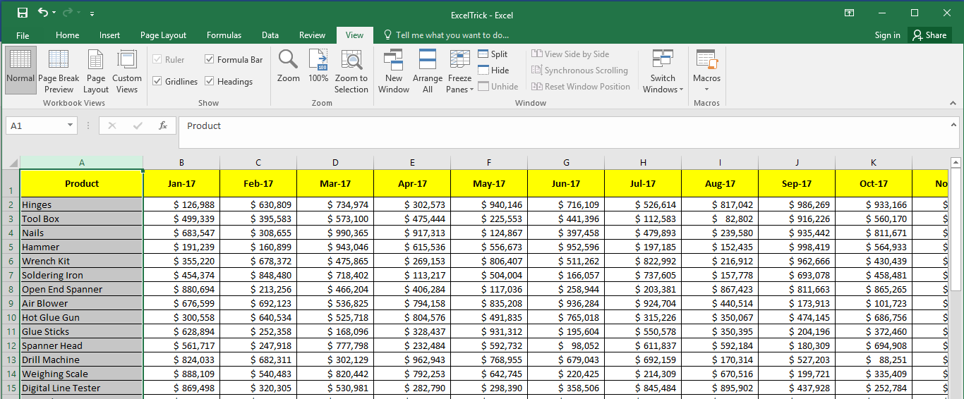
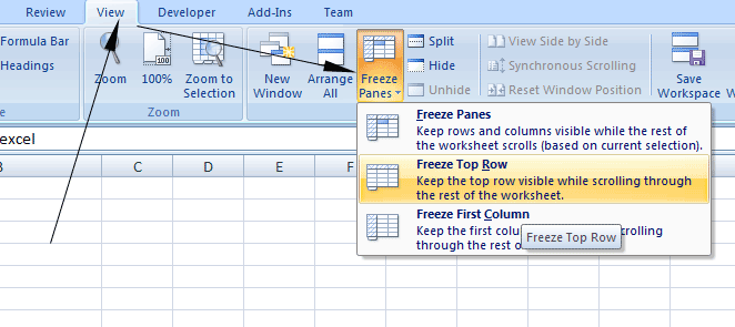
- Now, navigate to the “View” tab in the Excel Ribbon as shown in above image
- Click on the “Freeze Panes” button
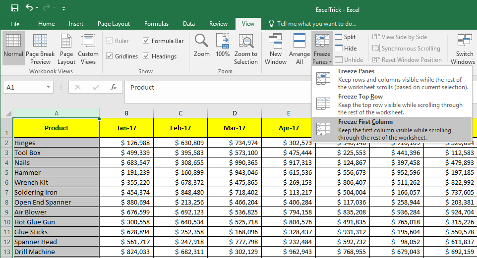
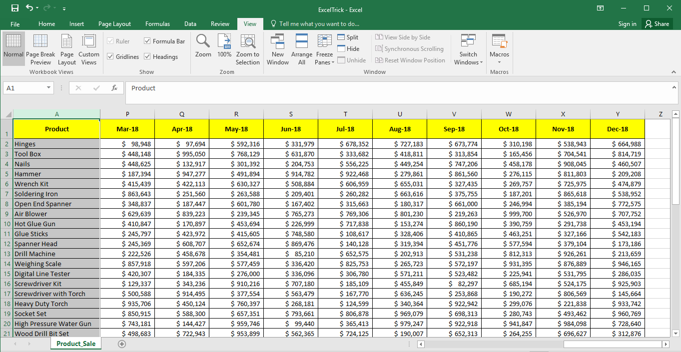
That’s it. You are all set now. As seen in above image you can now move to most right corner of the page and you would see that the first column sticks there. Please note that this option works as long as first column in excel is the one that you really want to freeze. If you have shifted right in the middle of the sheet and Column M is appearing as first row, then this option would freeze Column M and not Column A.
If you would like to do it directly using a keyboard shortcut, then please press “Alt + W” followed by “F” and then “C”. Please note that this is not an in-built shortcut, rather it’s the same thing from keyboard as we do from mouse.
Freeze All Worksheets Macro
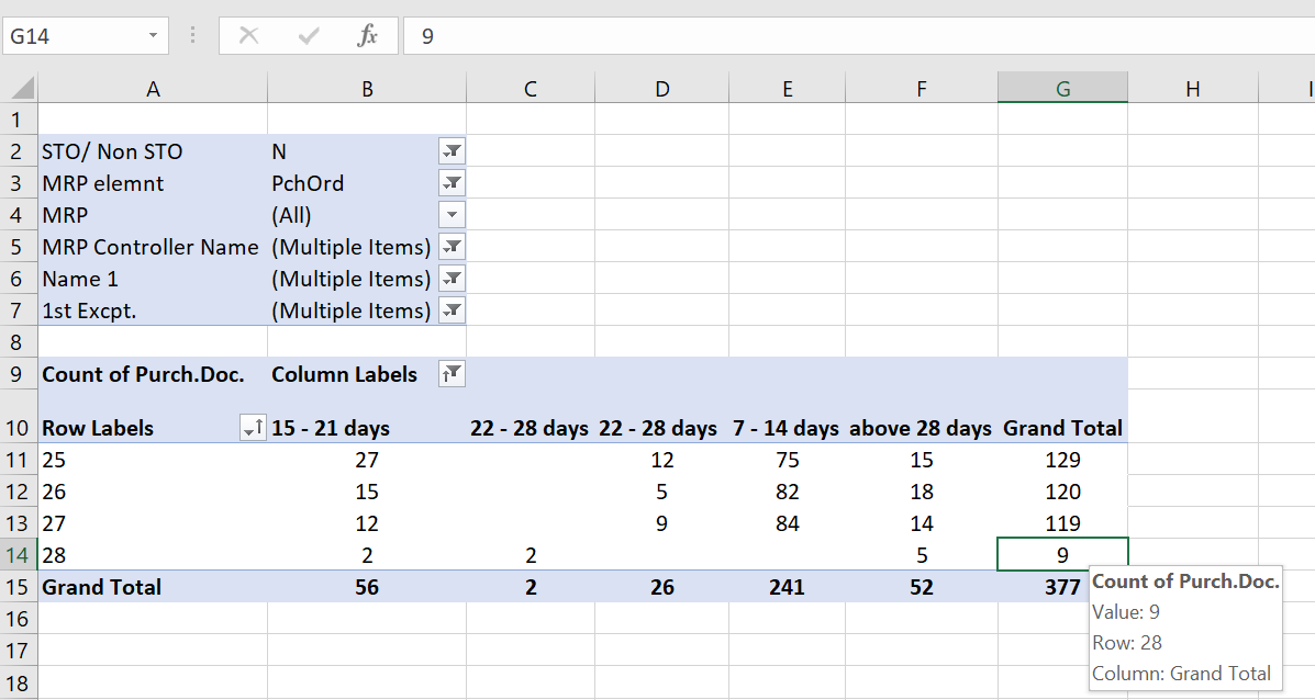
Use this macro to freeze all the sheets in the active workbook. Before you run the macro, select a cell, row or column, below and to the right of the area that you want frozen. See details in the chart in the previous section.
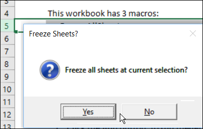
When the macro starts, it will show a confirmation message. Click Yes to go ahead with the unfreezing, and click No to cancel. In this screen shot, row 5 is selected, so rows 1 to 4 will be frozen on all sheets, if the Yes button is clicked.
Copy this macro into a regular code module, then select cell(s) on any worksheet, and run the macro to freeze all the sheets.
Sub FreezeAllSheets()
'www.contextures.com
Dim wsA As Worksheet
Dim ws As Worksheet
Dim wbA As Workbook
Dim strSel As String
Dim lRsp As Long
On Error GoTo errHandler

Set wbA = ActiveWorkbook
Set wsA = ActiveSheet
strSel = Selection.Address

lRsp = MsgBox("Freeze all sheets at current selection?", _
  vbQuestion + vbYesNo + vbDefaultButton1, "Freeze Sheets?")

If lRsp = vbYes Then
  Application.ScreenUpdating = False
  For Each ws In wbA.Worksheets
    ws.Activate
    Range(strSel).Select
    ActiveWindow.FreezePanes = True
  Next ws
  wsA.Activate
Else
  'do nothing
End If

exitHandler:
  Application.ScreenUpdating = True
  Exit Sub
errHandler:
  MsgBox "Could not freeze all sheets"
  Resume exitHandler

End Sub
Freeze Rows and Columns with a Keyboard Shortcut
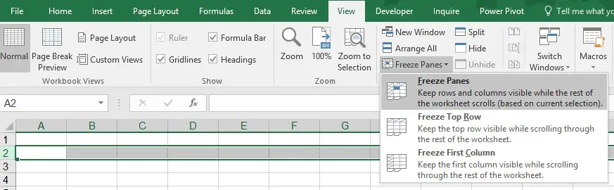
There is no dedicated keyboard shortcut for freezing panes in Excel, but you can access the commands with the Alt hotkeys.
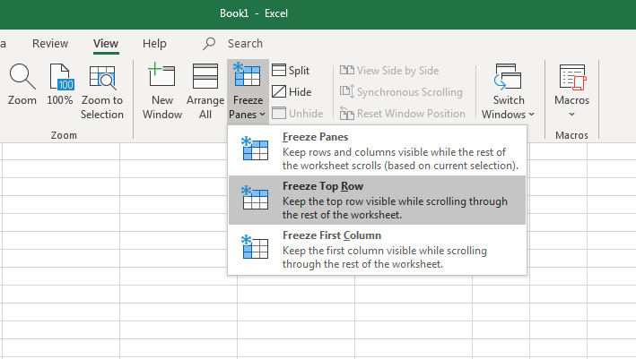
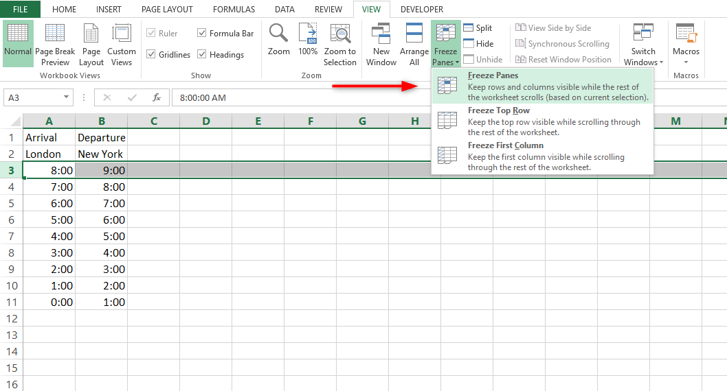
Press the sequence Alt, W, F and this will open the Freeze Panes menu in the View tab. Then you can use the following keys.
- Press the F key to Freeze Panes. This acts as a toggle and will also unfreeze the rows or columns if they are already frozen.
- Press the R key to Freeze Top Row.
- Press the C key to Freeze First Column.
When using the Freeze Panes shortcut, remember to select the cell directly below and to the right of the rows and columns you want to be frozen.
Note: When using the Freeze Panes shortcut, remember to select the cell directly below and to the right of the rows and columns you want to be frozen.
Unfreeze All Worksheets Macro
Use this macro to unfreeze all the sheets in the active workbook. It doesn’t matter which worksheet or which cell is selected before you run this macro.
When the macro starts, it will show a confirmation message. Click Yes to go ahead with the unfreezing, and click No to cancel.
Copy this macro into a regular code module, and run the macro to unfreeze all the sheets.
Sub UnfreezeAllSheets()
'www.contextures.com
Dim wsA As Worksheet
Dim ws As Worksheet
Dim wbA As Workbook
Dim lRsp As Long
On Error GoTo errHandler

Set wbA = ActiveWorkbook
Set wsA = ActiveSheet

lRsp = MsgBox("Unfreeze all sheets?", _
  vbQuestion + vbYesNo + vbDefaultButton1, "Unfreeze Sheets?")

If lRsp = vbYes Then
  Application.ScreenUpdating = False
  For Each ws In wbA.Worksheets
    ws.Activate
    ActiveWindow.FreezePanes = False
  Next ws
  wsA.Activate
Else
  'do nothing
End If

exitHandler:
  Application.ScreenUpdating = True
  Exit Sub
errHandler:
  MsgBox "Could not unfreeze all sheets"
  Resume exitHandler

End Sub
How do I stop VBA from not responding in Excel?
You can stop a macro by holding the “Ctrl” button and pressing the “Break” button.
How do I stop a VBA macro from running?
To break the running VBA program, do one of the following:
- On the Run menu, click Break.
- On the toolbar, click “Break Macro” icon.
- Press Ctrl + Break keys on the keyboard.
- Macro Setup > Stop (E5071C measurement screen)
- Press Macro Break key on the E5071C front panel.
How do I undo a macro after running?
In fact, running a macro completely erases the Undo list, and therefore you cannot automatically undo the effects of running the macro. There is no intrinsic command—in Excel or in VBA—to preserve the Undo list.
Why is undo not working in Excel?
Try saving and closing your Excel file, then re-opening in “Safe Mode.” I am assuming you are running VBA in the model, and the macros are disrupting the redo/undo functionality. “Safe Mode” disables the macros… check to see if you can undo/redo then check back…
Can you undo VBA code?
1 Answer. It can only undo the last action taken by the user and cannot undo VBA commands.
How do I redo a macro in Excel?
You might have noticed the Undo (Ctrl+Z) and Redo (Ctrl+Y) buttons usually lose their previous “stack” of choices whenever you run an Excel macro. You might subsequently notice the Repeat button (also Ctrl+Y) repeats the Excel macro that was recently run.
How do I undo clear content in Excel?
joeu2004. undone by ctrl-Z in Excel.
How do I undo a macro in Word?
Remove a macro in Word
- In Word, press Alt + F8 keys together to activate the Macros dialog.
- Other methods to activate the Macros dialog:
- In the Macros dialog, please select the macro you want to remove, and click the Delete button.
- Now in the Microsoft Word dialog, please click the Yes button to go ahead.
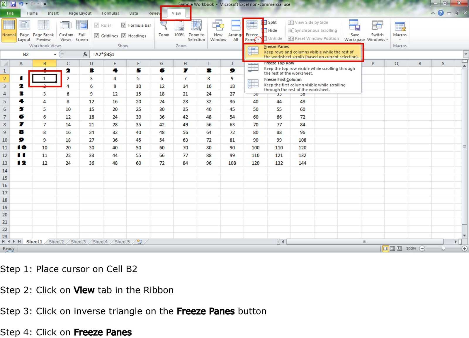
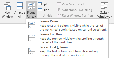
Freeze Panes
This feature could be used to freeze multiple rows, columns or both at the same time. However, this could be done only for the consecutive rows or columns.
Freeze Panes – Multiple Rows
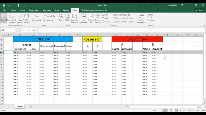
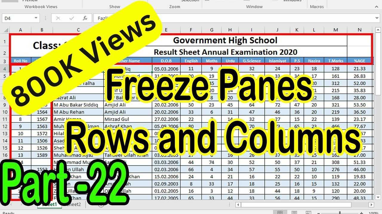
Open the sheet where in you want to freeze the multiple rows, keep the first row on top and click after the last row till where you want to freeze, as an example we would like to freeze from Row 1 to Row 13 so we will click on Row 14
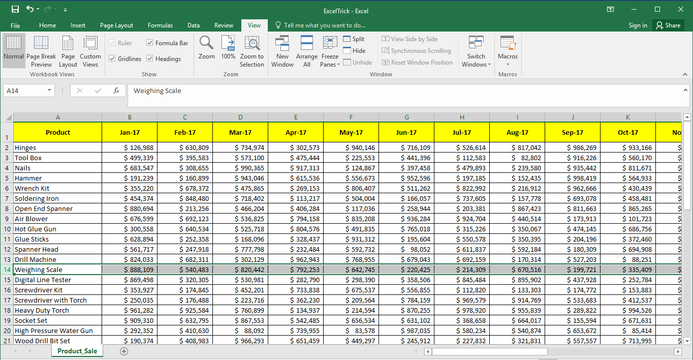
- Now, navigate to the “View” tab in the Excel Ribbon as shown in above image
- Click on the “Freeze Panes” button
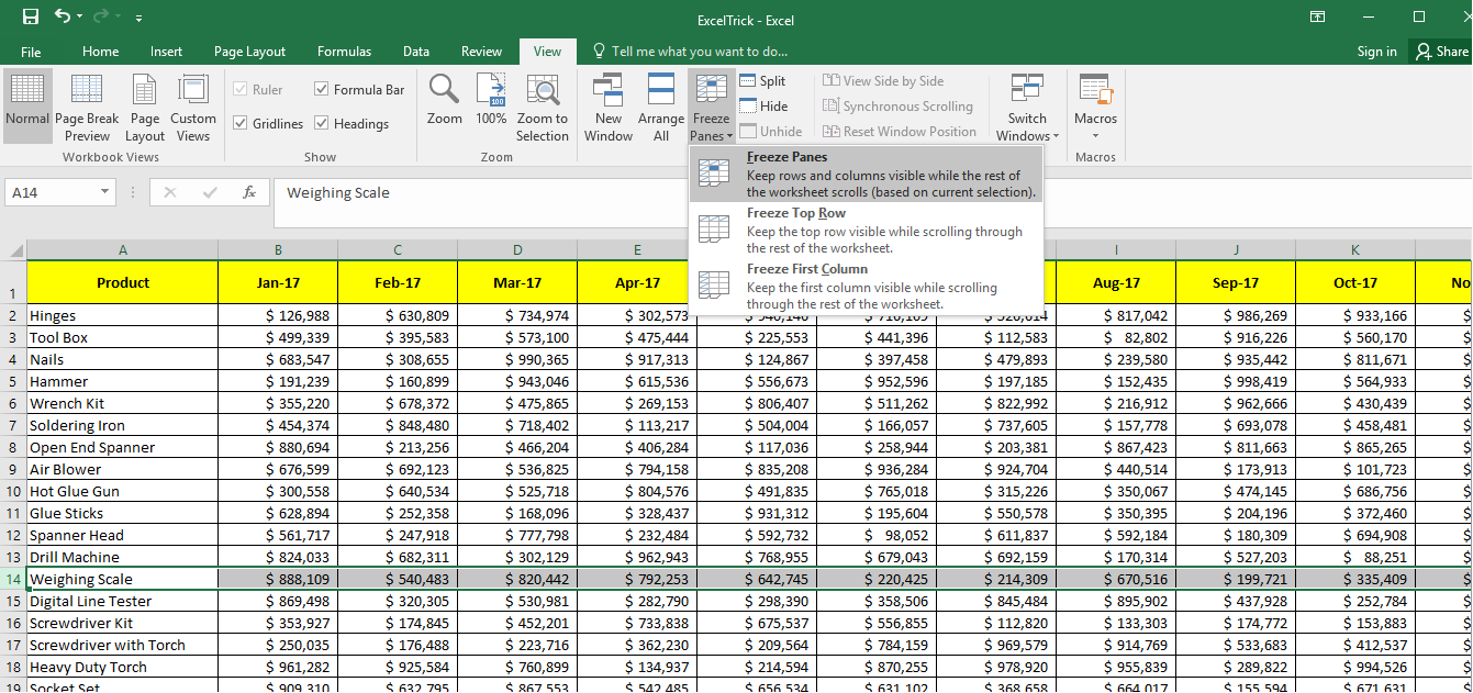
That’s it. You are all set now. As seen in above image you can now scroll down and Row 1 to Row 13 will be kept intact without any changes. You can select the range of rows from middle as well like – Row 13 to Row 30, however to do so you will have to ensure that you scroll up and keep Row 13 as your first row in the sheet and repeat the steps listed above. However, be careful as doing so some of your rows (i.e. the ones before Row 13) will be hidden.

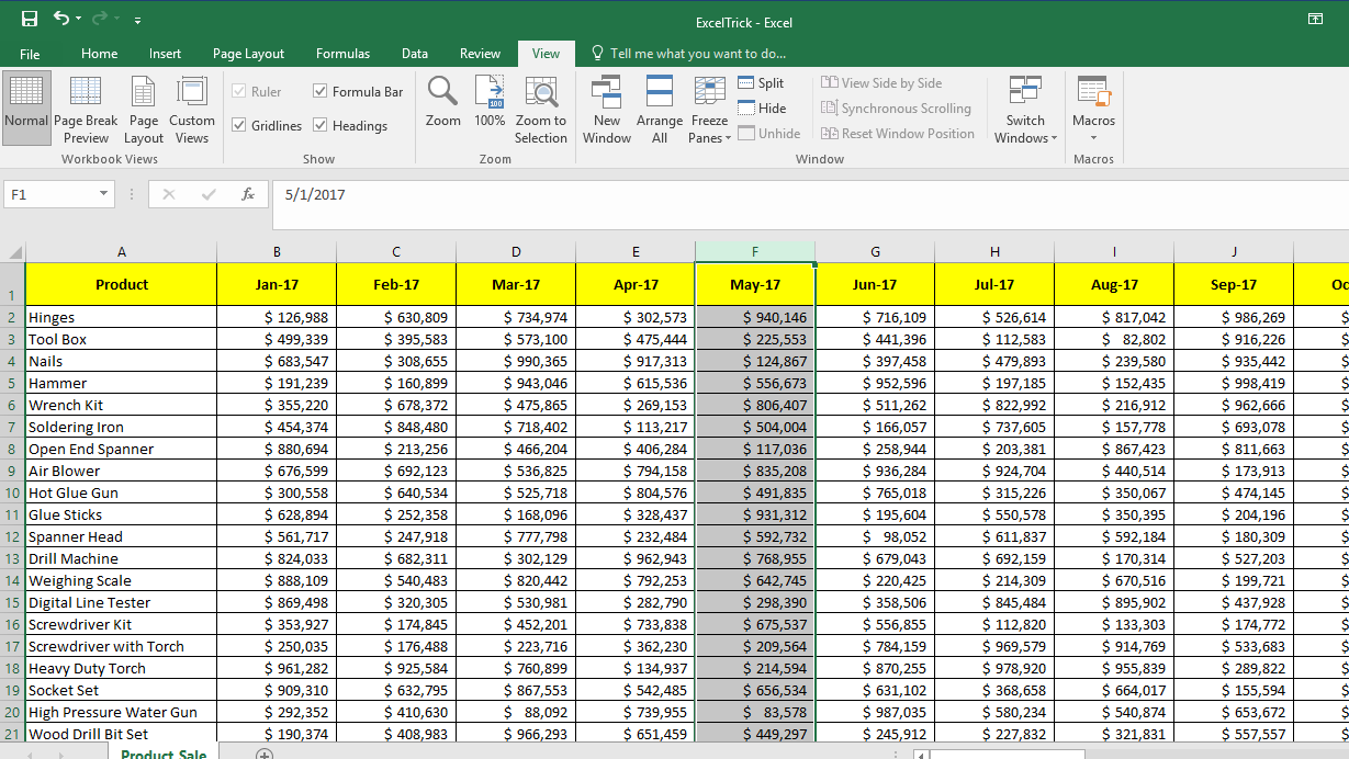
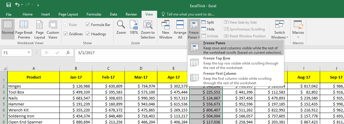
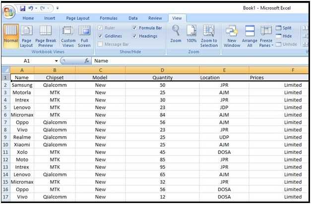
Freeze Panes – Multiple Columns
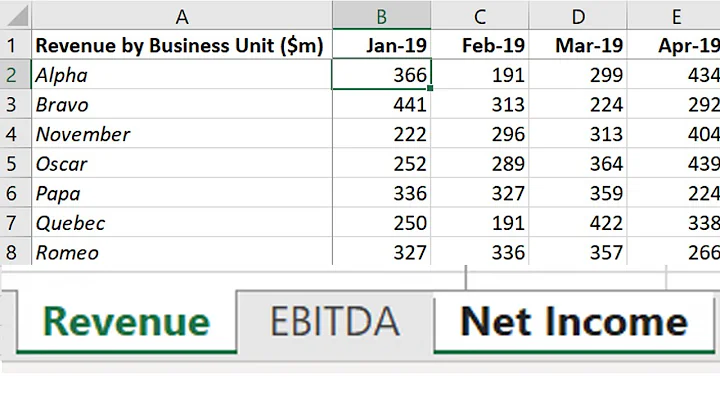
Open the sheet where in you want to freeze the multiple columns, keep the first column to the left and click next to the last column till where you want to freeze, as an example we would like to freeze from Column A to E, so we will click on Column F
- Now, navigate to the “View” tab in the Excel Ribbon as shown in above image
- Click on the “Freeze Panes” button
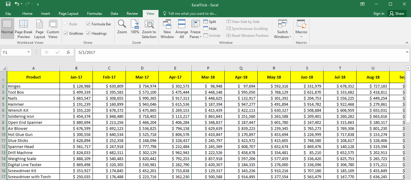
That’s it. You are all set now. As seen in above image you can now move towards right and Column A to E will be kept intact without any changes. You can select the range of columns from middle as well like – Column F to Column L, however to do so you will have to ensure that you move to the left and keep Column F as your first column in the sheet and repeat the steps listed above. However, be careful as doing so some of your columns (i.e. the ones before Column E) will be hidden.
Freeze Panes – Multiple Rows and Columns both
If you have followed the post till now, then you would have already figured out how this has to be done. Yes, you are right we are going to club both the above listed approaches here. Follow us below:
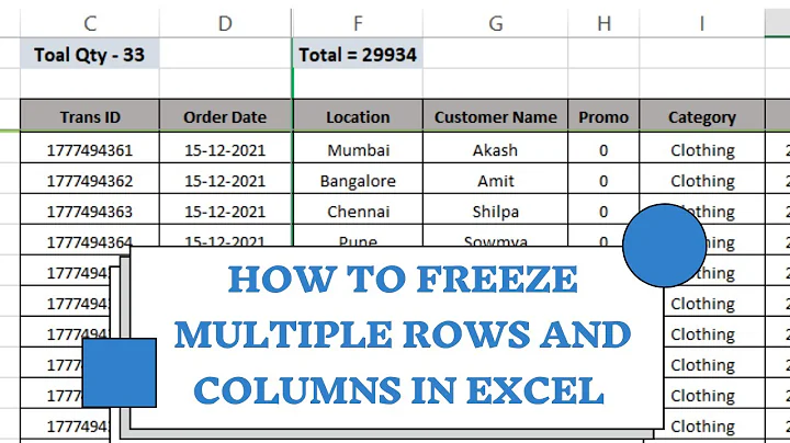
Open the sheet where in you want to freeze the multiple rows and columns, keep the first row on top and first column to the left then click next to the cell of the last column and row till where you want to freeze, as an example we would like to freeze from Row 1 to 13 and Column A to E, so we will click on Cell F14
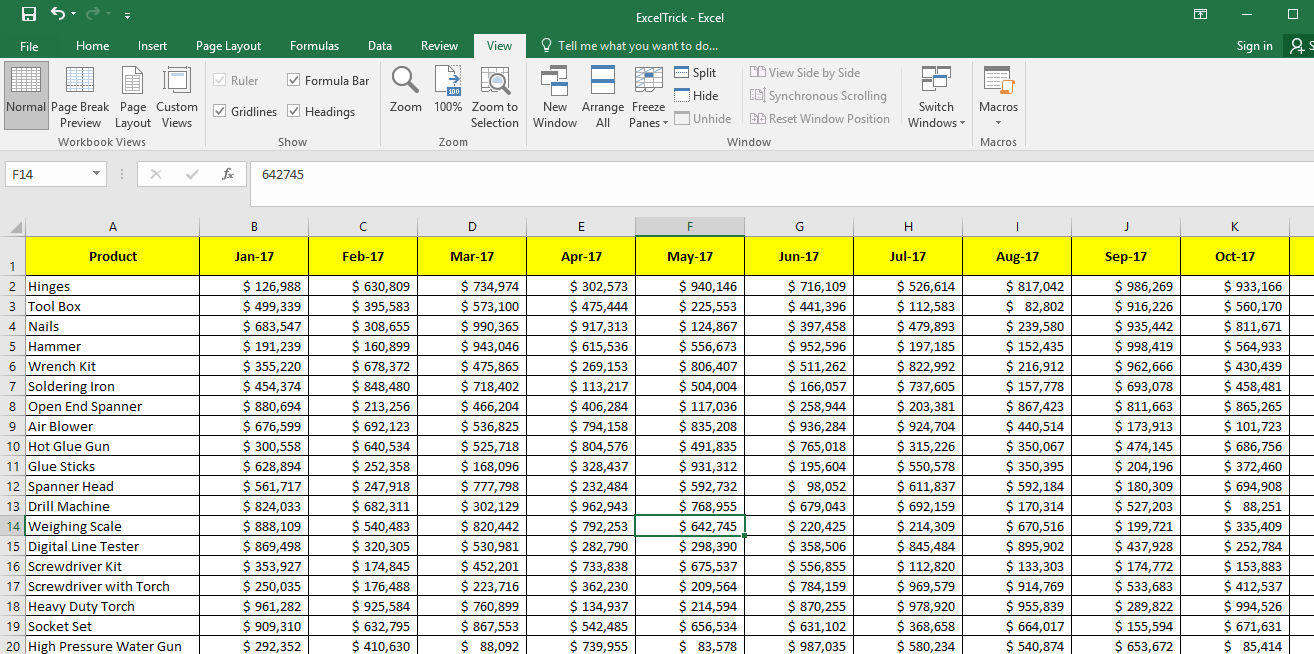
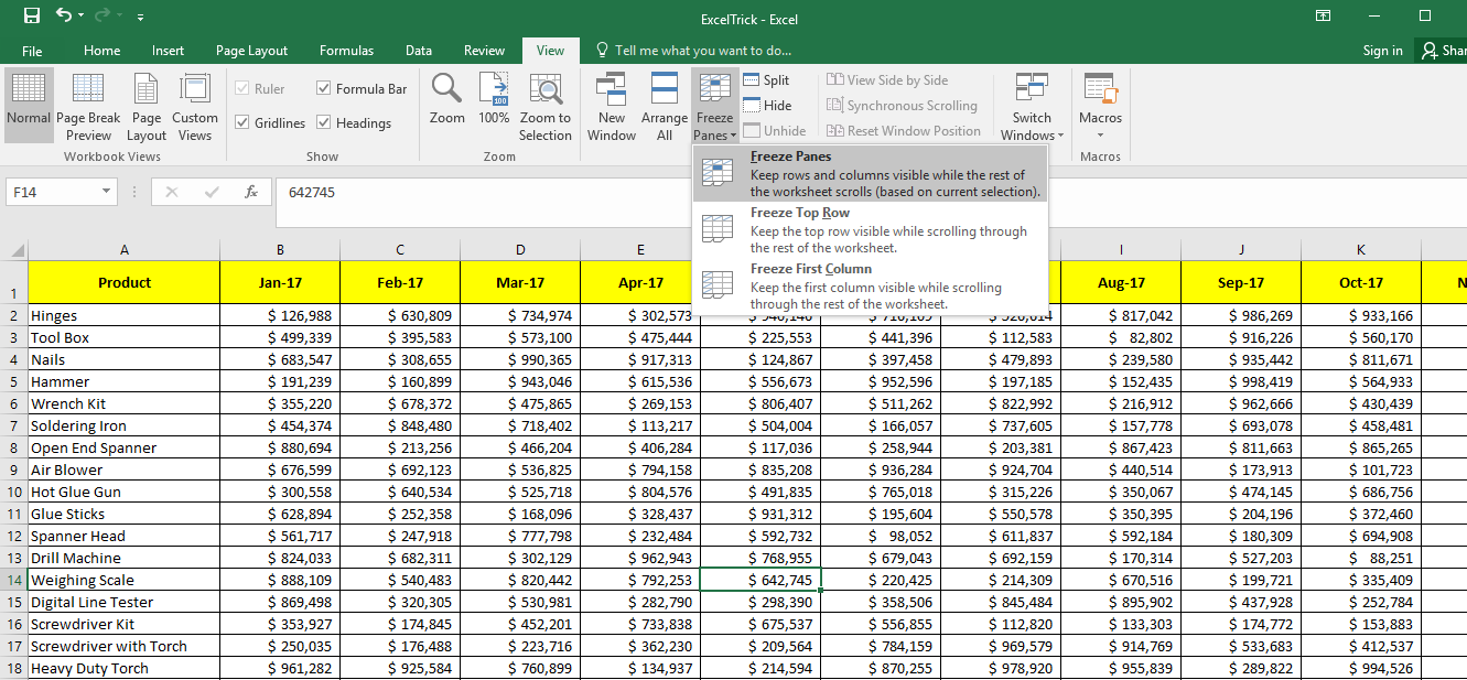
- Now, navigate to the “View” tab in the Excel Ribbon as shown in above image
- Click on the “Freeze Panes” button
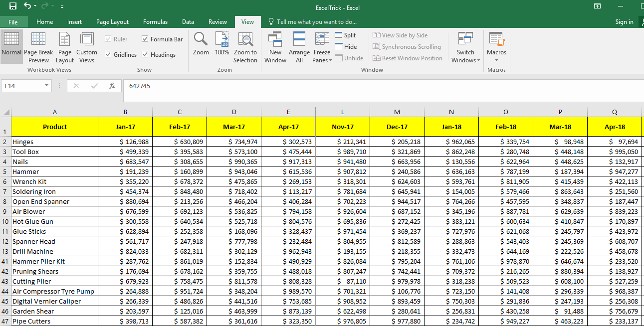
That’s it. You are all set now. As seen in above image you can now scroll down and Row 1 to 13 will remain intact and likewise you can move towards right and Column A to E will be kept intact without any changes. You can select the range of columns from middle as well like – Row 17 to 27 and Column F to L, however to do so you will have to ensure that you scroll up and keep Row 17 as your first row and keep Column F as your first column in the sheet and repeat the steps listed above. Be careful here as rows before Row 17 and columns before column F will be hidden.
Другие способы закрепления ячеек
В предыдущем разделе мы рассмотрели простой способ закрепления ячеек с помощью VBA Excel. Однако, в Excel существуют и другие способы закрепления ячеек, которые также могут быть полезными при работе с большими наборами данных.
1. Использование функции ЗАКРЕПИТЬ
Функция ЗАКРЕПИТЬ позволяет закрепить ячейки простым способом без использования VBA кода. Для этого необходимо выделить ячейки, которые нужно закрепить, затем щелкнуть правой кнопкой мыши на выделенной области и выбрать пункт «Закрепить ячейки». После этого выбранные ячейки останутся видимыми при прокрутке таблицы, в то время как остальные ячейки будут скрыты.
Примечание: функция ЗАКРЕПИТЬ доступна только в некоторых версиях Excel и может иметь ограничения по количеству закрепленных ячеек.
2. Использование функции ЗАМОРОЗКА ОКНА
Функция ЗАМОРОЗКА ОКНА также позволяет задать закрепление ячеек без использования VBA кода. Для этого необходимо выбрать ячейку, с которой начнется закрепление, затем перейти на вкладку «Вид» в главном меню Excel и выбрать пункт «Заморозить окно». Следующий шаг — выбрать ячейку, после которой закрепление будет прекращено. После этого при прокрутке таблицы первые строка или столбец будут оставаться на своем месте, а остальные строки или столбцы будут прокручиваться.
Примечание: функция ЗАМОРОЗКА ОКНА также имеет некоторые ограничения, включая возможность закрепления только первой строки или первого столбца.
Помимо перечисленных выше функций, существуют и другие способы закрепления ячеек в Excel, включая использование различных команд и настроек в VBA. Знание этих способов позволит вам упростить работу с данными и повысить эффективность работы с Excel.
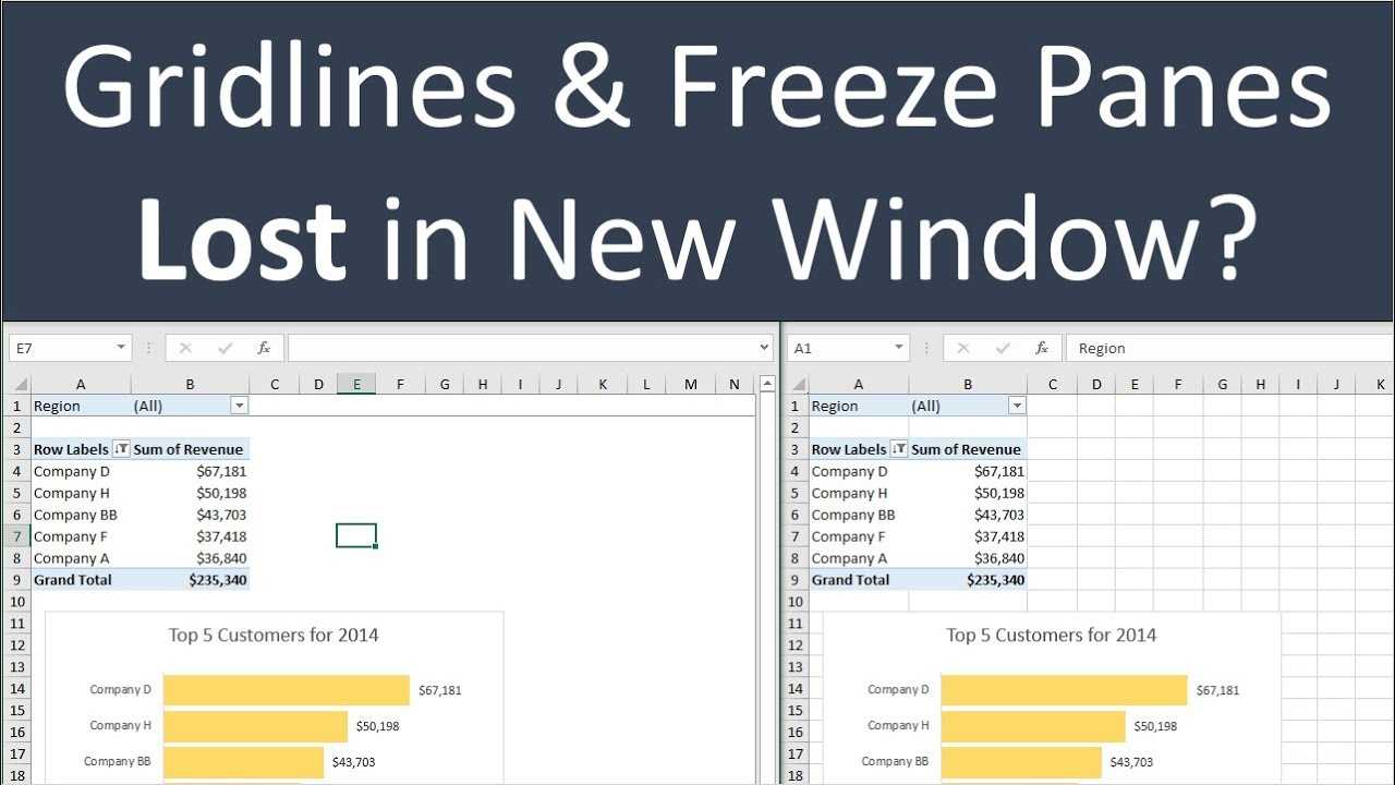
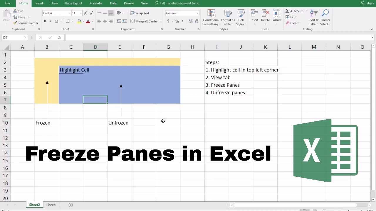
What Is Freeze Panes In Excel?
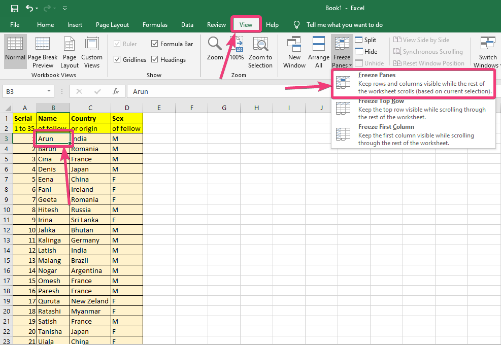
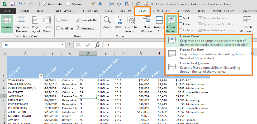
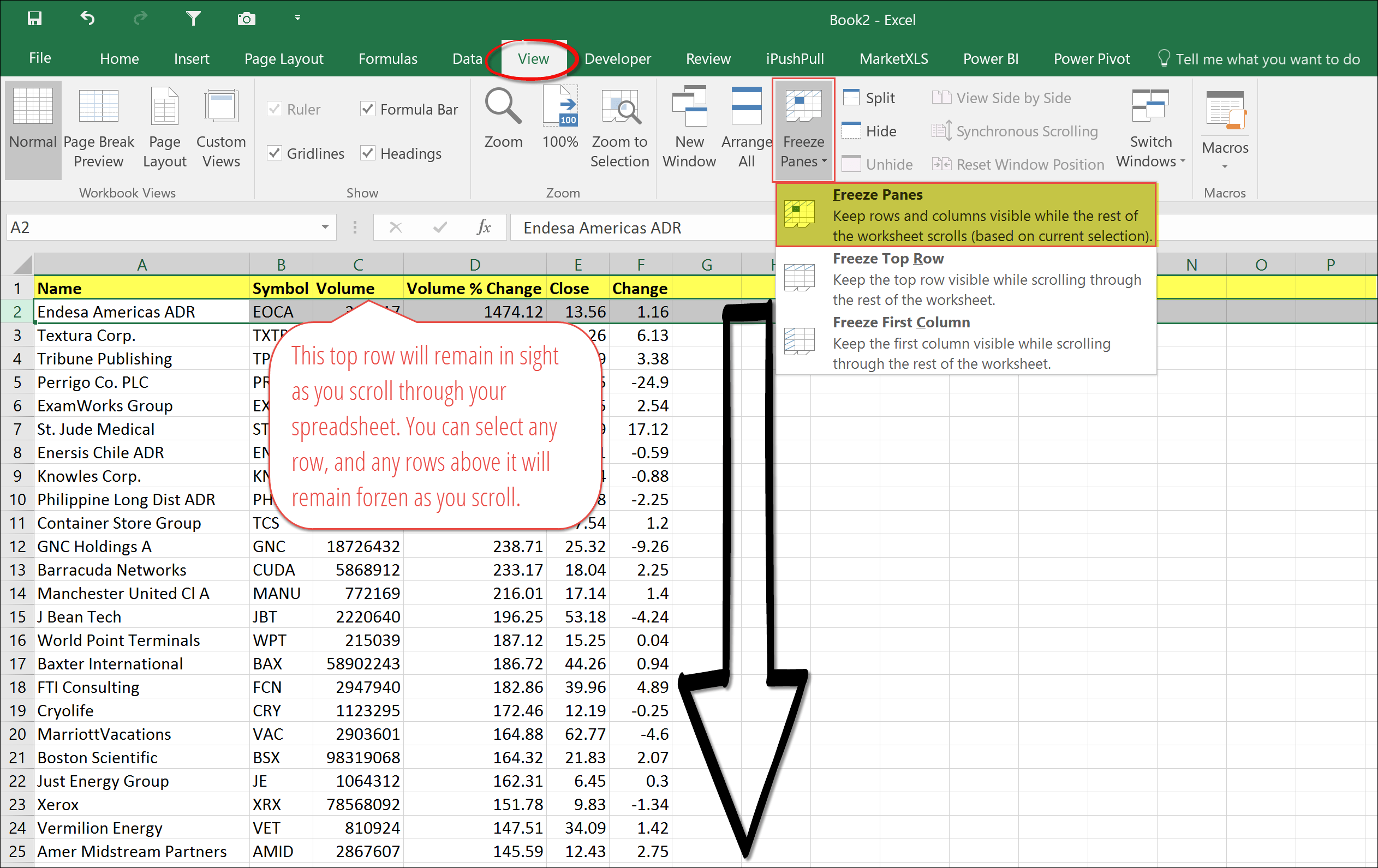
Excel Freeze Panes option is used to lock row or column headings. So that when you scroll down or view the rest portions of the sheet its top row or first column gets stick on the screen.
In this way, heading will always appear no matter how you scroll in your worksheet.
Freezing the pane headings is a very helpful feature mainly when you work with the table having information that crosses the columns and rows appearing onscreen.
For more clear idea of this specific excel problem, check out this user query.
To extract data from corrupt Excel file, we recommend this tool:
This software will prevent Excel workbook data such as BI data, financial reports & other analytical information from corruption and data loss. With this software you can rebuild corrupt Excel files and restore every single visual representation & dataset to its original, intact state in 3 easy steps:
- Try Excel File Repair Tool rated Excellent by Softpedia, Softonic & CNET.
- Select the corrupt Excel file (XLS, XLSX) & click Repair to initiate the repair process.
- Preview the repaired files and click Save File to save the files at desired location.
Users Query Regarding Freeze Panes Not Working
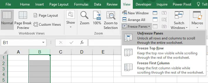
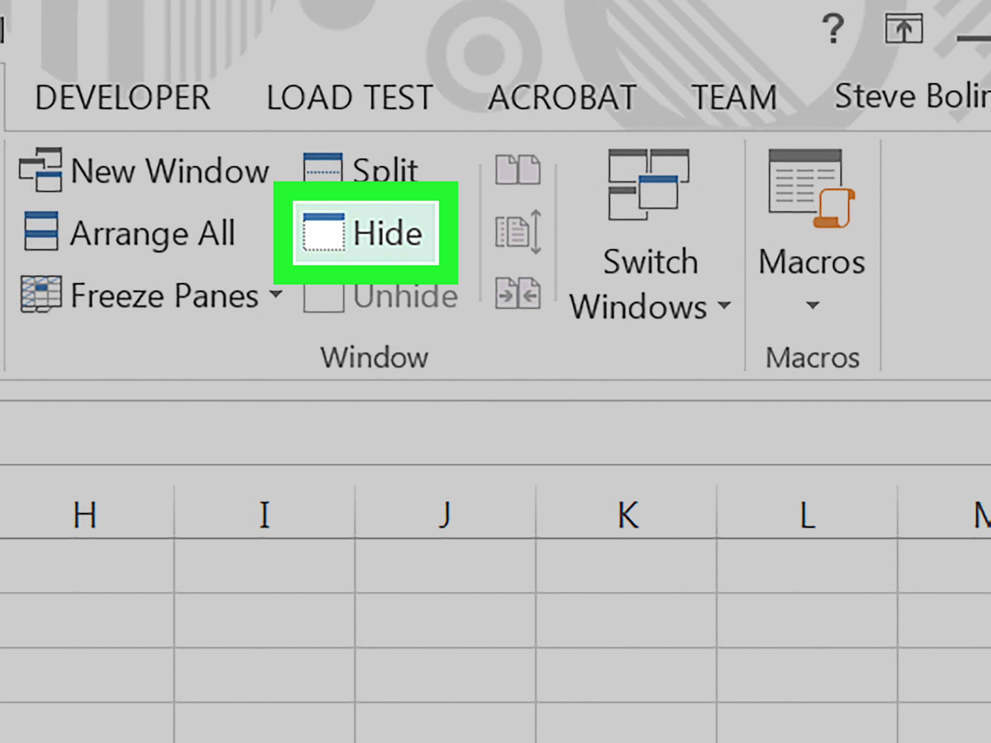
Unfreeze Panes:
If you have frozen the wrong rows and columns, then you could easily undo it by using “Unfreeze Panes” option. This would remove all the frozen rows and \ or columns in your excel. This will also work if you have received the sheet from someone else and you are not able to see all the rows and columns despite of removing all filters and unhiding rows \ columns. To unfreeze panes –
- Open the sheet wherein you want to unfreeze rows and \ or columns
- Now, navigate to the “View” tab in the Excel Ribbon
- Click on the “Freeze Panes” button
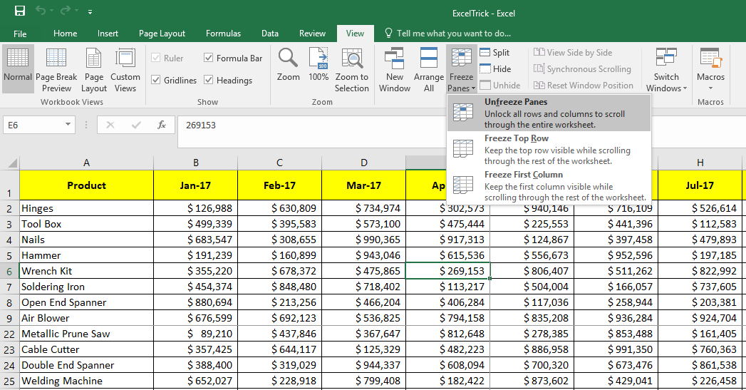
With this all the rows and \ or columns would unfreeze, as shown in above image. Please note that you would not see the “Unfreeze Panes” option if there are not any frozen rows \ columns. This option would be available only and only when there is some row and \ or column frozen already.
If you would like to unfreeze panes it directly using a keyboard shortcut, then please press “Alt + W” followed by “F” and then again “F”. Please note that this is not an in-built shortcut, rather it’s the same thing from keyboard as we do from mouse.
Шаг 4: Установка параметров для ActiveWindow.FreezePanes
После того, как вы установили фиксацию панели с помощью метода ActiveWindow.FreezePanes, вы можете настроить параметры для этой функции. Эти параметры определяют, какая часть таблицы должна оставаться видимой, а какая будет прокручиваться вместе с содержимым окна.
Чтобы установить параметры для фиксации панели, вам понадобится использовать свойство ActiveWindow.SplitColumn и ActiveWindow.SplitRow.
- ActiveWindow.SplitColumn: Это свойство позволяет установить количество столбцов, которые будут закреплены слева от разделительной линии. Значение должно быть указано в виде положительного числа. Например, если вы хотите закрепить первые 3 столбца, вы должны установить значение SplitColumn равным 3.
- ActiveWindow.SplitRow: Это свойство позволяет установить количество строк, которые будут закреплены над разделительной линией. Значение также должно быть указано в виде положительного числа. Например, если вы хотите закрепить первые 2 строки, вы должны установить значение SplitRow равным 2.
Ниже приведен пример кода, показывающего, как установить значения SplitColumn и SplitRow:
Вы можете изменять значения SplitColumn и SplitRow в соответствии со своими потребностями. После установки параметров вызовите метод FreezePanes, чтобы активировать фиксацию панели со всеми настроенными параметрами.
В результате активное окно Excel будет иметь закрепленные столбцы и строки, которые будут оставаться на месте при прокрутке содержимого окна.
Freeze Panes with Office Scripts
If you are using Excel online with a Microsoft 365 business plan, then you will be able to automate your tasks with Office Scripts.
This is a JavaScript based language currently only available in the web version of Excel.
You can use Office Scripts to quickly loop through all your sheets and freeze panes in them.
Go to the Automate tab and click on the New Script command. This will open up the Code Editor and you can copy and paste the above code into it.
Press the Save script button and then press the Run button.
The code will turn the freeze panes option on across all the sheets in the workbook.
️ Warning: When you Freeze Panes from the user interface, you need to select the cell directly below and to the right of the rows and columns to freeze. But this works differently in the Office Scripts code. The method requires the selection to be on the last row and column to freeze!
Solution 3
I need to be able to properly refreeze panes (when creating new windows, notably) without losing the activecell or messing up the visible range. It took a lot of playing around but I think I have something solid that works:
Solution 4
The problem with splitting is that if a user unfreezes panes, the panes will remain split. (I couldn’t find a way to turn off split afterwards while keeping the panes frozen)
This may be too obvious/simple, but what if the current selection is simply saved and then re-selected afterwards?
Solution 5
I know this is old but I came across this tidbit that may be useful…
as ChrisB stated, the SplitColumn/SplitRow values represent the last cell above/left of the split BUT of the currently visible window. So if you happen to have code like this:
The split will be between rows 110 and 111 instead of 10 and 11.
edited for clarification and to add more information:
My point is that the values are offsets of the upper left cell, not an address of a cell. Therefore, ChrisB’s Dec 4 ’15 at 18:34 comment under the main answer only holds if row 1 is visible in the Activewindow.
A couple of other points on this:
- using Application.goto doesn’t necessarily put whichever cell you
are trying to go to in the upper left - the cell that is put in the upper left when using .goto can depend
on the size of the excel window, the current zoom level, etc (so fairly arbitrary) - it is possible to have the splits placed so that you can not see
them or even scroll around in the visible window (if .FreezePanes =
true). for example:
CETAB may be dealing with this in their answer.
81,127
Related videos on Youtube
 07 : 38
Freeze panes across selected sheets
Strategize Financial Modelling
297
 03 : 36
How to Freeze Panes in Excel
Kevin Stratvert
124
 02 : 39
— MS Excel — Freeze Pane freezes too many rows — freezes half of the sheet
Alro Developers
18
 02 : 36
How to Freeze Multiple Rows and Columns in Excel Using Freeze Panes (Lock Rows and Columns in Excel)
ZSF TECHOOK
11
 03 : 12
Excel VBA code for Freeze Panes
Chester Tugwell
4
 47 : 12
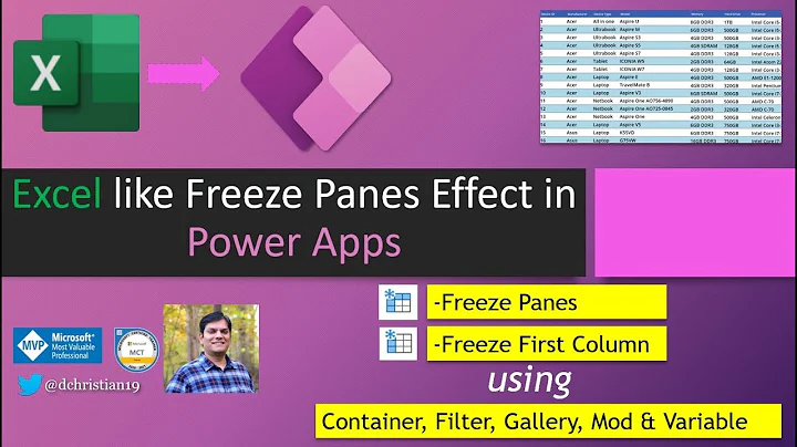
Excel like freeze panes effect in Power Apps
Daniel Christian
3
 02 : 01
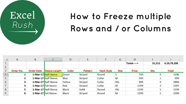
How to Freeze Multiple Rows and or Columns in Excel using Freeze Panes
Excel Rush .com
1
-
ChrisB
almost 2 yearsI have a VBA script in Excel that freezes the panes of an Excel worksheet, but I’m curious to see if this is possible without first selecting a range. Here’s by code now which freezes rows 1 through 7:
Any suggestions?
-
Tuntable
about 5 yearsDoes not make sense. Seems to work OK, even if referenced window is not active.
-
ChrisB
about 2 yearsFor a more accurate comparison, freeze panes on separate sheets instead of over and over on the same worksheet. Any real world use of freezing panes many times would involve separate sheets. (I can think of one real world example: a large number of reports generated for different users.) Also, your method doesn’t un-freeze panes first, so if panes were already frozen, even in a different location on the sheet, it doesn’t do anything. I suspect the time was so fast because no actions were completed for loops 2–1000 but I’m curious to see if that’s actually true.
-
pstraton
over 1 yearYes, this type of technique is the most reliable with the least unwanted side effects. (See my comment above, regarding user4039065‘s post.) But I would also set ActiveWindow.FreezePanes = False before selecting cell A2, in case Freeze Panes is already set to some other state, which would prevent this code from producing the desired effect.
-
pstraton
over 1 yearAlso, beware: instead of Range(«A2»).Select, it may be tempting to to do something like Range(«1:1»).Select or Rows(1).Select, but doing so actually creates a quad-window freeze-panes state. (With no apparent usefulness, so maybe an old Excel bug?)
Solution 5
I know this is old but I came across this tidbit that may be useful…
as ChrisB stated, the SplitColumn/SplitRow values represent the last cell above/left of the split BUT of the currently visible window. So if you happen to have code like this:
The split will be between rows 110 and 111 instead of 10 and 11.
edited for clarification and to add more information:
My point is that the values are offsets of the upper left cell, not an address of a cell. Therefore, ChrisB’s Dec 4 ’15 at 18:34 comment under the main answer only holds if row 1 is visible in the Activewindow.
A couple of other points on this:
- using Application.goto doesn’t necessarily put whichever cell you
are trying to go to in the upper left - the cell that is put in the upper left when using .goto can depend
on the size of the excel window, the current zoom level, etc (so fairly arbitrary) - it is possible to have the splits placed so that you can not see
them or even scroll around in the visible window (if .FreezePanes =
true). for example:
CETAB may be dealing with this in their answer.
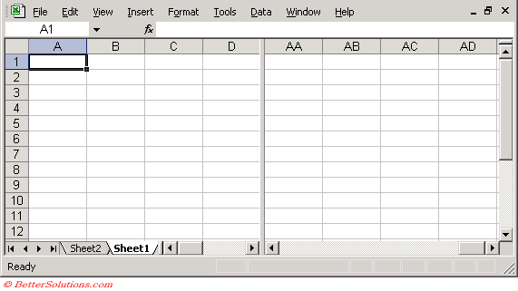
Freeze panes versus Splitting Panes:
Excel also provides you an excellent option to Split Panes which divides the window into different panes that each pane scrolls separately. This option is present in Excel Ribbon, View tab next to Freeze Option.
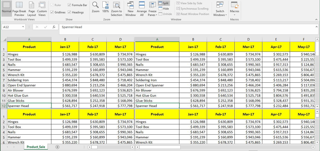
So as visible in the above image after using split option the content of same sheet is visible in 4 separate panes and all panes have their different scroll options.
We personally trust and use Freeze option much than Split, as Freeze allows you to limit the data movement by freezing it rather than adding multiple views of same data wherein you easily get distracted and confused while data entry.
What This VBA Code Does
I hate changing the Freeze Pane location because it takes two steps instead of one. You first have to remove the current Freeze Pane and then turn it back on to your new preferred location. This inspired me to create a simple VBA macro that would do both of these steps with the click of a button. This code will also remove the freeze panes if you run it with the current freeze panes cell intersection selected (giving you a toggle on/off feature). Enjoy!

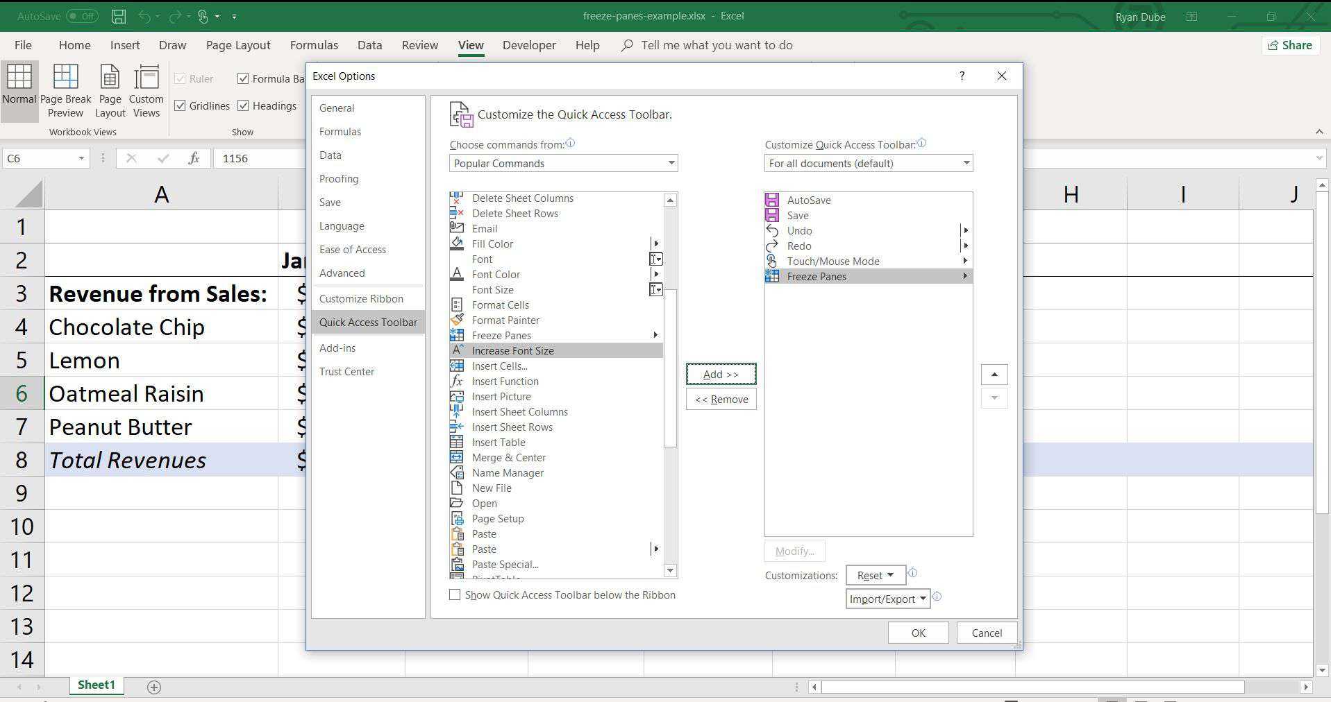
Using VBA Code Found On The Internet
Now that you’ve found some VBA code that could potentially solve your Excel automation problem, what do you do with it? If you don’t necessarily want to learn how to code VBA and are just looking for the fastest way to implement this code into your spreadsheet, I wrote an article (with video) that explains how to get the VBA code you’ve found running on your spreadsheet.
Getting Started Automating Excel
Are you new to VBA and not sure where to begin? Check out my quickstart guide to learning VBA. This article won’t overwhelm you with fancy coding jargon, as it provides you with a simplistic and straightforward approach to the basic things I wish I knew when trying to teach myself how to automate tasks in Excel with VBA Macros.
Also, if you haven’t checked out Excel’s latest automation feature called Power Query, I have put together a beginner’s guide for automating with Excel’s Power Query feature as well! This little-known built-in Excel feature allows you to merge and clean data automatically with little to no coding!
How Do I Modify This To Fit My Specific Needs?
Chances are this post did not give you the exact answer you were looking for. We all have different situations and it’s impossible to account for every particular need one might have. That’s why I want to share with you: My Guide to Getting the Solution to your Problems FAST! In this article, I explain the best strategies I have come up with over the years to get quick answers to complex problems in Excel, PowerPoint, VBA, you name it!
I highly recommend that you check this guide out before asking me or anyone else in the comments section to solve your specific problem. I can guarantee that 9 times out of 10, one of my strategies will get you the answer(s) you are needing faster than it will take me to get back to you with a possible solution. I try my best to help everyone out, but sometimes I don’t have time to fit everyone’s questions in (there never seem to be quite enough hours in the day!).
I wish you the best of luck and I hope this tutorial gets you heading in the right direction!
Hidden Hacks For VBA Macro Coding
After 10+ years of creating macros and developing add-ins, I’ve compiled all the hacks I wish I had known years ago!
Learn These Hacks Now For Free!

Chris Newman
Chris is a finance professional and Excel MVP recognized by Microsoft since 2016. With his expertise, he founded TheSpreadsheetGuru blog to help fellow Excel users, where he shares his vast creative solutions & expertise. In addition, he has developed over 7 widely-used Excel Add-ins that have been embraced by individuals and companies worldwide.
Преимущества использования VBA
Одно из главных преимуществ использования VBA в Excel — это возможность создания пользовательских макросов, которые могут выполнять сложные операции автоматически. Это особенно полезно, когда необходимо обработать большое количество данных или выполнить серию действий, которые могут занимать значительное время при ручной обработке.
Также, использование VBA позволяет создавать пользовательские функции, которые могут быть использованы для расчетов, обработки данных или построения отчетов. Это дает возможность создавать более сложные и гибкие формулы, которые превосходят стандартные функции Excel.
Еще одним преимуществом использования VBA является возможность работы с объектной моделью Excel. С помощью VBA можно автоматически создавать, редактировать и форматировать книги Excel, рабочие листы, графики и диаграммы. Это позволяет создавать кастомизированные решения, специально разработанные под конкретные бизнес-задачи.
Кроме того, VBA обладает широкими возможностями для обработки и анализа данных. С его помощью можно осуществлять сортировку, фильтрацию, поиск и замену данных, а также создавать сложные отчеты и диаграммы.
Наконец, использование VBA позволяет повысить надежность и безопасность работы с данными в Excel. Макросы и пользовательские функции, созданные на VBA, могут быть защищены паролем и ограничены доступом только для определенных пользователей. Это обеспечивает конфиденциальность и предотвращает нежелательные изменения данных или кода.
В целом, использование VBA в Excel предоставляет широкие возможности для автоматизации задач, обработки и анализа данных, а также создания кастомизированных решений под конкретные бизнес-задачи. Однако, для успешного использования VBA необходимо иметь хотя бы базовые знания программирования и понимание работы с объектной моделью Excel.