Описание метода pastespecial вба excel

Заметки

NoHTMLFormatting имеет значение только при формате = «HTML»; во всех остальных случаях NoHTMLFormatting игнорируется.

Перед использованием этого метода необходимо выбрать диапазон назначения.

Этот метод может изменять выбор листа в зависимости от содержимого буфера обмена.

Для разработчиков языков, помимо английского, можно заменить одну из следующих констант (0-5), чтобы соответствовать строковому эквиваленту формата файла изображений.

Аргумент Format	Эквивалент строки
«Изображение (PNG)»
1	«Изображение (JPEG)»
2	«Изображение (GIF)»
3	«Picture (Enhanced Metafile)»
4	«Bitmap»
5	«Microsoft Office объект рисования»

Openpyxl iterate by rows

The function return cells from the worksheet as rows.

iterating_by_rows.py

#!/usr/bin/python

from openpyxl import Workbook

book = Workbook()
sheet = book.active

rows = (
    (88, 46, 57),
    (89, 38, 12),
    (23, 59, 78),
    (56, 21, 98),
    (24, 18, 43),
    (34, 15, 67)
)

for row in rows:
    sheet.append(row)

for row in sheet.iter_rows(min_row=1, min_col=1, max_row=6, max_col=3):
    for cell in row:
        print(cell.value, end=" ")
    print()

book.save('iterbyrows.xlsx')

The example iterates over data row by row.

for row in sheet.iter_rows(min_row=1, min_col=1, max_row=6, max_col=3):

We provide the boundaries for the iteration.

$ ./iterating_by_rows.py
88 46 57
89 38 12
23 59 78
56 21 98
24 18 43
34 15 67

Copy / Paste formatting only shortcut

First let’s go over an example of how to use the keyboard shortcut to copy / paste format only. This is the easiest way to copy formatting in your spreadsheet. First you use the normal keyboard shortcut to copy a selection (Ctrl + C), and then you use a special keyboard shortcut to paste only the formatting, as shown below.

Keyboard shortcuts for pasting formatting only in Google Sheets:

Ctrl + Alt + V (Windows or Chrome OS)

⌘ + Option + V (Mac)

To copy and paste formatting only in Google sheets, follow these steps:

1. Select the cell or range of cells that contains the formatting that you want to copy
2. Press Ctrl + C on the keyboard to copy the selection
3. Select the cell where you want to paste the formatting into
4. Press Ctrl + Alt + V on the keyboard to paste the formatting only (⌘ + Option + V for Mac)

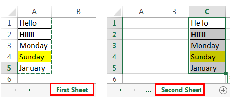
In this example we have student data in cells that have been formatted in several ways, such as fill color, font size, and bold font.

We are going to copy the formatting from the left side of the sheet, to the right side of the sheet, so that the right side of the sheet is formatted exactly like the left side is. In this case we are going to paste the formatting only, without transferring the values and formulas from the cells.

To do this we will use the keyboard shortcut to copy the cells and then paste format only.

First we select the range A1:C5. Then press Ctrl + C on the keyboard.

As you can see in the image below, the range A1:C5 has been copied. The blue dotted lines that appear around the range indicate that the selection is copied.

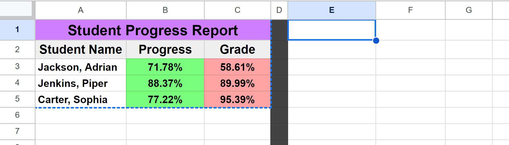
Cell E1 is selected, which is where we are going to paste the formatting. When you are pasting multiple cells, select the first cell that is in the range that you want to paste into (the cell that is on the top left of the range to be pasted into).

Then press Ctrl + Alt + V on the keyboard to paste only the formatting without the values and the formulas (⌘ + Option + V for Mac)

As you can see in the image below, after using the paste formatting shortcut, the formatting from the range A1:C5 has now been copied into the range A1:G5.

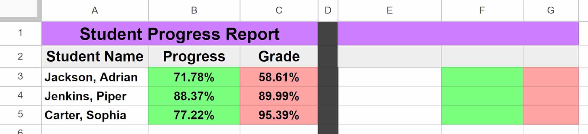
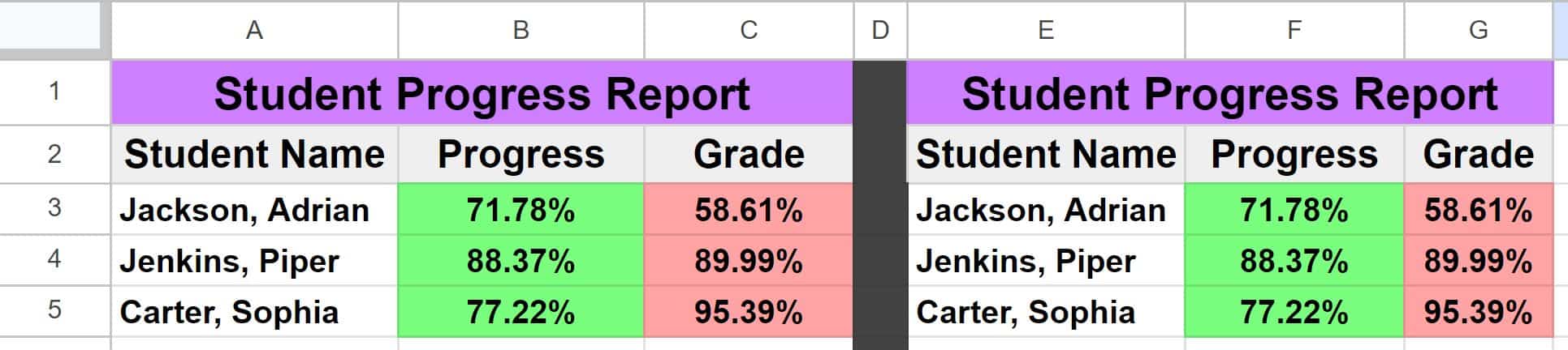
In this case the cells in the range E1:G5 do not contain any values, and initially you can see that the fill color formatting has been transferred. But in the image below you can see that after values are entered into the cells, the text and numbers also match the format from the range A1:C5.

Check out this article if you want to learn how to paste values only, without formulas or formatting.

Formatting a single cell vs. a range of cells vs. columns and rows

You can copy formatting from a single cell to another cell, or from a range of cells to another range of cells.

When using any of the methods in this lesson to copy formatting, when you first select a range of cells before copying the formatting, the same size of range will be affected when you paste the formatting.

If you select a range that is three cells wide by three cells tall, when you copy the formatting from that range to another location in the spreadsheet it will affect a range three cells wide and three cells tall, making it match the original selected range.

As you will learn later in the lesson, if you select entire columns or rows before copying the formatting, when you paste the format the width of the columns and the height of the rows will be transferred as well.

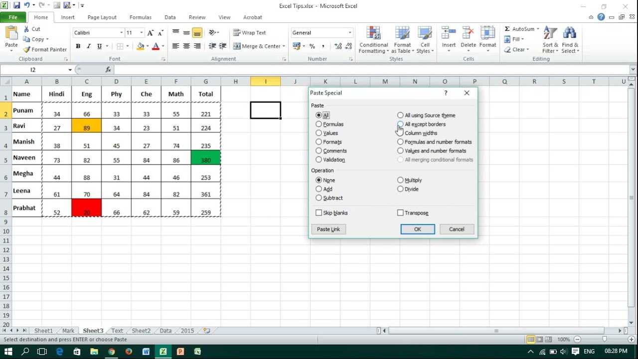
Range.PasteSpecial method

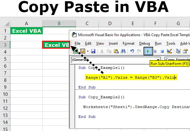
When working with your spreadsheet, you likely often have to copy formulas and paste them as values. To do this in a macro, you can use the PasteSpecial method.

Parameters

Name	Required/Optional	Data type	Description
Paste	Optional	XlPasteType	Specifies the part of the range to be pasted.
Operation	Optional	XlPasteSpecialOperation	Specifies how numeric data will be calculated with the destinations cells on the worksheet.
SkipBlanks	Optional	Variant	True to have blank cells in the range on the clipboard not be pasted into the destination range. The default value is False.
Transpose	Optional	Variant	True to transpose rows and columns when the range is pasted. The default value is False.

XlPasteType enumeration

Name	Value	Description
xlPasteAll	-4104	Everything will be pasted.
xlPasteAllExceptBorders	7	Everything except borders will be pasted.
xlPasteAllMergingConditionalFormats	14	Everything will be pasted and conditional formats will be merged.
xlPasteAllUsingSourceTheme	13	Everything will be pasted using the source theme.
xlPasteColumnWidths	8	Copied column width is pasted.
xlPasteComments	-4144	Comments are pasted.
xlPasteFormats	-4122	Copied source format is pasted.
xlPasteFormulas	-4123	Formulas are pasted.
xlPasteFormulasAndNumberFormats	11	Formulas and Number formats are pasted.
xlPasteValidation	6	Validations are pasted.
xlPasteValues	-4163	Values are pasted.
xlPasteValuesAndNumberFormats	12	Values and Number formats are pasted.

XlPasteSpecialOperation enumeration

Name	Value	Description
xlPasteSpecialOperationAdd	2	Copied data will be added to the value in the destination cell.
xlPasteSpecialOperationDivide	5	Copied data will divide the value in the destination cell.
xlPasteSpecialOperationMultiply	4	Copied data will multiply the value in the destination cell.
xlPasteSpecialOperationNone	-4142	No calculation will be done in the paste operation.
xlPasteSpecialOperationSubtract	3	Copied data will be subtracted from the value in the destination cell.

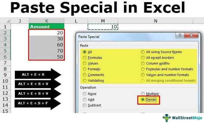
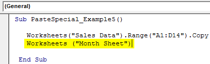
Example 5: Multiply

This example replaces the data in cells on Sheet1 with the multiply of the existing contents and cells on Sheet1.

1 2	A B C D 1 2 3 3 4 5 6

VBA Code

Result

1 2	A B C D 3 6 9 3 12 15 18

Example 6: Add

This example replaces the data in cells on Sheet1 with the sum of the existing contents and cells on Sheet1.

1 2	A B C D 1 2 3 3 4 5 6 3

VBA Code

Result

1 2	A B C D 1 2 3 4 4 5 6 7

Openpyxl formulas

The next example shows how to use formulas. The does not
do calculations; it writes formulas into cells.

formulas.py

#!/usr/bin/python

from openpyxl import Workbook

book = Workbook()
sheet = book.active

rows = (
    (34, 26),
    (88, 36),
    (24, 29),
    (15, 22),
    (56, 13),
    (76, 18)
)

for row in rows:
    sheet.append(row)

cell = sheet.cell(row=7, column=2)
cell.value = "=SUM(A1:B6)"
cell.font = cell.font.copy(bold=True)

book.save('formulas.xlsx')

In the example, we calculate the sum of all values with the
function and style the output in bold font.

rows = (
    (34, 26),
    (88, 36),
    (24, 29),
    (15, 22),
    (56, 13),
    (76, 18)
)

for row in rows:
    sheet.append(row)

We create two columns of data.

cell = sheet.cell(row=7, column=2)

We get the cell where we show the result of the calculation.

cell.value = "=SUM(A1:B6)"

We write a formula into the cell.

cell.font = cell.font.copy(bold=True)

We change the font style.Figure: Calculating the sum of values

Специализированные параметры PasteSpecial

Метод PasteSpecial в VBA Excel предоставляет возможность копирования и вставки специальных форматов данных. Помимо стандартных параметров, таких как замена значения, форматирование ячеек и т.д., PasteSpecial предлагает ряд специализированных опций. Рассмотрим их подробнее:

1. Add — при вставке, каждое число будет добавлено к соответствующей ячейке в диапазоне. Это полезно, когда необходимо добавить значения из одного диапазона к другому.

2. Subtract — каждое число в диапазоне будет вычтено из соответствующей ячейки в выбранном диапазоне. Используется, когда необходимо вычесть значения из другого диапазона.

3. Multiply — каждое число в диапазоне будет умножено на соответствующую ячейку в выбранном диапазоне. Это полезно для умножения значений в разных диапазонах.

4. Divide — каждая ячейка в выбранном диапазоне будет разделена на соответствующее число в исходном диапазоне. Используется для деления значений.

5. Transpose — вставка данных из исходного диапазона в ячейки переворачивается. То есть, если исходные данные находятся в столбце, они будут вставлены в строку и наоборот.

6. Values — копируются только значения из исходного диапазона. Форматирование, формулы и другие атрибуты не сохраняются.

7. Formats — копируются только форматы ячеек, без значений и формул.

8. Comments — копируются только комментарии, оставленные в исходном диапазоне.

9. Validation — копируются только условное форматирование, установленное в исходном диапазоне.

10. AllUsingSourceTheme — копируются значения, форматирование и стили ячеек так, как они выглядят в исходном диапазоне.

11. AllExceptBorders — копируются значения, форматирование, формулы и прочие атрибуты ячеек за исключением границ.

12. AllUsingDestinationTheme — копируются значения, форматирование и стили ячеек так, как они выглядят в целевом диапазоне.

13. AllMergingConditionalFormats — копируются значения и объединение условного форматирования из исходного диапазона в целевой.

14. ColumnWidths — копируются ширина столбцов.

15. Formulas — копируются только формулы из исходного диапазона.

16. FormulasAndNumberFormats — копируются формулы и форматы чисел. Это полезно, если вам нужно скопировать как значения, так и формулы одновременно.

Если вы используете метод PasteSpecial с определенными параметрами, убедитесь, что вы правильно выбрали целевой диапазон для вставки данных. В противном случае, произойдет перезапись существующих данных или другие нежелательные эффекты могут возникнуть.

Параметр	Описание
Add	Добавляет значения из исходного диапазона к соответствующим ячейкам в целевом диапазоне.
Subtract	Вычитает значения из исходного диапазона из соответствующих ячеек в целевом диапазоне.
Multiply	Умножает значения из исходного диапазона на соответствующие ячейки в целевом диапазоне.
Divide	Делит значения из исходного диапазона на соответствующие ячейки в целевом диапазоне.
Transpose	Переворачивает данные из исходного диапазона при вставке в целевой диапазон.
Values	Копирует только значения из исходного диапазона без форматирования и формул.
Formats	Копирует только форматы ячеек без значений и формул.
Comments	Копирует только комментарии из исходного диапазона.
Validation	Копирует только условное форматирование из исходного диапазона.
AllUsingSourceTheme	Копирует значения, форматирование и стили ячеек из исходного диапазона.
AllExceptBorders	Копирует значения, форматирование, формулы и прочие атрибуты ячеек, за исключением границ.
AllUsingDestinationTheme	Копирует значения, форматирование и стили ячеек из исходного диапазона, так, как они выглядят в целевом диапазоне.
AllMergingConditionalFormats	Копирует значения и объединяет условное форматирование из исходного диапазона в целевой.
ColumnWidths	Копирует ширину столбцов из исходного диапазона.
Formulas	Копирует только формулы из исходного диапазона.
FormulasAndNumberFormats	Копирует формулы и форматы чисел из исходного диапазона.

Final Verdict:

Whether you are using PC or phone clipboard is always an essential part of the ecosystem. Isn’t it..?

It runs in the background so that all your copy and paste works smoothly in your Excel application. All in all, this entire native feature is a much-needed boost and no one can bear error in this clipboard.

So without wasting any more time just try the above-listed fixes to easily get rid of there’s a problem with the clipboard Excel error.

Priyanka Sahu

Priyanka is a content marketing expert. She writes tech blogs and has expertise in MS Office, Excel, and other tech subjects. Her distinctive art of presenting tech information in the easy-to-understand language is very impressive. When not writing, she loves unplanned travels.

Pasting a Single Cell Value to All the Visible Rows of a Filtered Column

When it comes to pasting to a filtered column, there may be two cases:

• You might want to paste a single value to all the visible cells of the filtered column.
• You might want to paste a set of values to visible cells of the filtered column.

For the first case, pasting into a filtered column is quite easy.

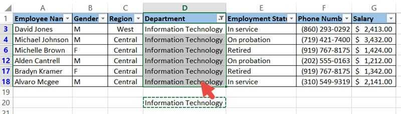
Let’s say we want to replace all the cells that have Department = “IT” with the full form: “Information Technology”.

For this, you can type the word “Information Technology” in any blank cell, copy it, and paste it to the visible cells of the filtered “Department” Column. Here’s a step-by-step on how to do this:

1. Select a blank cell and type the words “Information Technology”.
2. Copy it by press CTRL+C or Right click->Copy.
3. Select all the visible cells in the column with the “Department” header.
4. Paste the copied value by pressing CTRL+V or Right click->Paste.

You will find the value “Information Technology” pasted to only the visible cells of the column “Department”.

To verify this, remove the filter by selecting the Data->Filter. Notice that all the other cells of the “Department” column remain unchanged.

Macros in Excel

It has become easier to do repeated Excel tasks using Macros written in VBA. We can write Macros to do a specific job, and the user can run them whenever required.

It makes it easier to do complex things several times over and over again. The macros need to be coded once and can be used infinite times. Remember, we should write Macros in such a way that enhances useability.

Try NOT to hardcode values in a Macro. It is ideal for taking inputs from the user to enhance useability.

If you are looking for VBA statements that allow you to copy the values from one column to another in Excel, you must be aware of the definition and usage of a Macro.

Macros in Microsoft Excel are an excellent feature that repeatedly automates your desired tasks. In short, a Macro is an action or a set of activities that the user records to run it frequently.

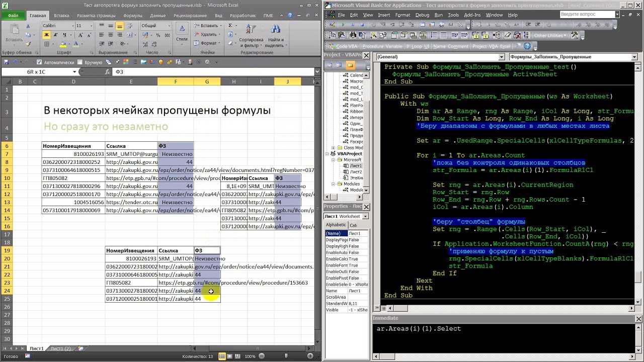
Изменение параметров Excel перед записью макросов

Завершить ввод данных в ячейки, если это не редактирование их содержимого, можно нажатием на самые различные клавиши: клавиши перемещения на одну ячейку (вниз, вверх, влево, вправо), Home, End, Page Up или Page Down . Самый же классический способ завершения ввода данных в Excel — нажатие на клавишу Enter , после чего, как правило, табличный курсор перемещается на ячейку ниже. И это довольно удобно. Большинство пользователей полагают, что это неизменяемое свойство Excel . На самом же деле этот параметр устанавливается при инсталляции Excel по умолчанию и при желании может быть изменен.

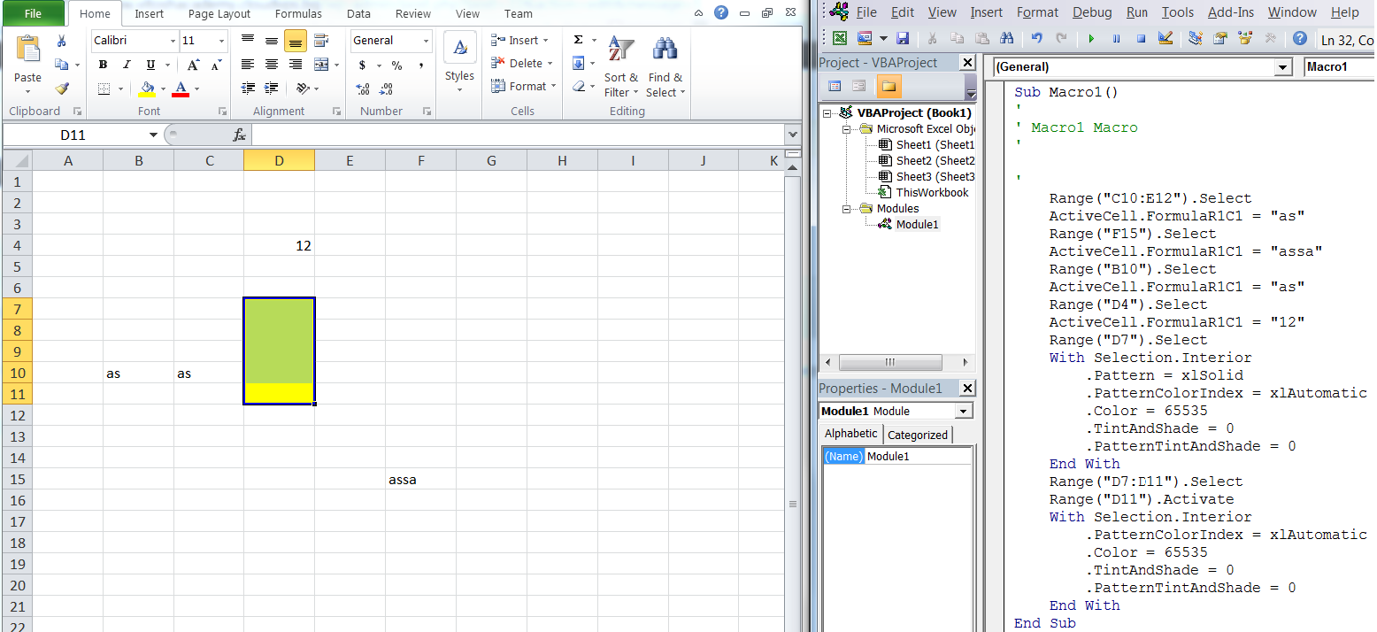
И если при работе по вводу данных непосредственно на рабочем листе, перемещение табличного курсора на ячейку ниже после фиксации ввода клавишей Enter — удобство, то при записи макроса — недостаток.

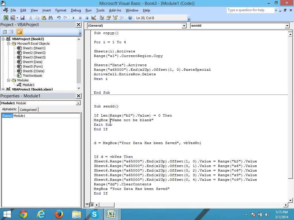
Недостаток заключается в том, что либо перед остановкой записи макроса или при проведении каких-либо других операций после ввода данных в ячейку (диапазон ячеек), адрес ячейки, в которой окажется табличный курсор, будет зафиксирован отдельной строкой кода VBA (см. рисунок 4).

В последующем, при выполнении записанного макроса, эта операция будет выполняться, как один из переходов на зафиксированную ячейку. Это увеличивает продолжительность выполнения макроса и «утяжеляет» файл Excel на количество символов этой строки. А при редактировании кода макроса в Редакторе Microsoft Visual Basic будет потрачено время на удаление этих строк.

Поэтому, прежде чем записывать макросы, связанные с операциями ввода данных, с помощью команды Сервис | Параметры откройте диалоговое окно Параметры и на вкладке Правка (рисунок 1) удалите флажок с опции Переход к другой ячейке после ввода .

Рис.1. Диалоговое окно Параметры , вкладка Правка с открытым раскрывающимся списком В направлении при активизированной опции Переход к другой ячейке после ввода

Иначе при записи макроса, перемещение табличного курсора после нажатия на клавишу Enter на ячейку, по заданному этой опцией в направлении, выбранном в раскрывающемся списке В направлении , будет отражено в сгенерированном коде макроса.

Merging cells

Cells can be merged with the method and unmerged with
the method. When we merge cells, all cells but the
top-left one are removed from the worksheet.

merging_cells.py

#!/usr/bin/python

from openpyxl import Workbook
from openpyxl.styles import Alignment

book = Workbook()
sheet = book.active

sheet.merge_cells('A1:B2')

cell = sheet.cell(row=1, column=1)
cell.value = 'Sunny day'
cell.alignment = Alignment(horizontal='center', vertical='center')

book.save('merging.xlsx')

In the example, we merge four cells: A1, B1, A2, and B2. The text in the final
cell is centered.

from openpyxl.styles import Alignment

In order to center a text in the final cell, we use the
class from the module.

sheet.merge_cells('A1:B2')

We merge four cells with the method.

cell = sheet.cell(row=1, column=1)

We get the final cell.

cell.value = 'Sunny day'
cell.alignment = Alignment(horizontal='center', vertical='center')

We set text to the merged cell and update its alignment.Figure: Merged cells

Работа с диапазоном в переменной

Работать с диапазоном в переменной можно точно также, как и с диапазоном на рабочем листе. Все свойства и методы объекта Range действительны и для диапазона, присвоенного переменной. При обращении к ячейке без указания свойства по умолчанию возвращается ее значение. Строки

равнозначны. В обоих случаях информационное сообщение MsgBox выведет значение ячейки с индексом 6.

Важно: если вы планируете работать только со значениями, используйте переменные массивов, код в них работает значительно быстрее. Преимущество работы с диапазоном ячеек в объектной переменной заключается в том, что все изменения, внесенные в переменной, применяются к диапазону (который присвоен переменной) на рабочем листе

Преимущество работы с диапазоном ячеек в объектной переменной заключается в том, что все изменения, внесенные в переменной, применяются к диапазону (который присвоен переменной) на рабочем листе.

Пример 1 — работа со значениями

Скопируйте процедуру в программный модуль и запустите ее выполнение.

Обратите внимание, что ячейки диапазона на рабочем листе заполнились так же, как и ячейки в переменной диапазона, что доказывает их непосредственную связь между собой

Пример 2 — работа с форматами

Продолжаем работу с тем же диапазоном рабочего листа «C6:E8»:

Опять же, обратите внимание, что все изменения форматов в присвоенном диапазоне отобразились на рабочем листе, несмотря на то, что мы непосредственно с ячейками рабочего листа не работали

Пример 3 — копирование и вставка диапазона из переменной

Значения ячеек диапазона, присвоенного переменной, передаются в другой диапазон рабочего листа с помощью оператора присваивания.

Скопировать и вставить диапазон полностью со значениями и форматами можно при помощи метода Copy, указав место вставки (ячейку) на рабочем листе.

В примере используется тот же диапазон, что и в первых двух, так как он уже заполнен значениями и форматами.

Информационное окно MsgBox добавлено, чтобы вы могли увидеть работу процедуры поэтапно, если решите проверить ее в своей книге Excel.

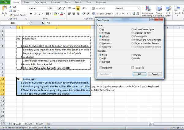
Paste Special from the Home Tab

If you’re not a keyboard person and prefer using the mouse, then you can access the Paste Values command from the ribbon commands.

Here’s how to use Paste Values from the ribbon.

1. Select and copy the data you want to paste into your clipboard.
2. Select the cell you want to copy the values into.
3. Go to the Home tab.
4. Click on the lower part of the Paste button in the clipboard section.
5. Select the Values clipboard icon from the paste options.

The cool thing about this menu is before you click on any of the commands you will see a preview of the data you’re about to paste. This makes it easy to ensure you’re selecting the right option.

Worksheet — Copy and Paste

1.0 The worksheet copy and paste sequence

In Excel, to copy and paste a range:

1. Select the source range
2. Copy the Selection to the Clipboard. Home > Clipboard > Copy, or Ctrl + C shortcut
3. Activate the target Worksheet
4. Select the upper left cell of target range
5. Paste from the Clipboard to the target range. Right Click > Paste, or Ctrl + V shortcut

In VBA, this is equivalent to:

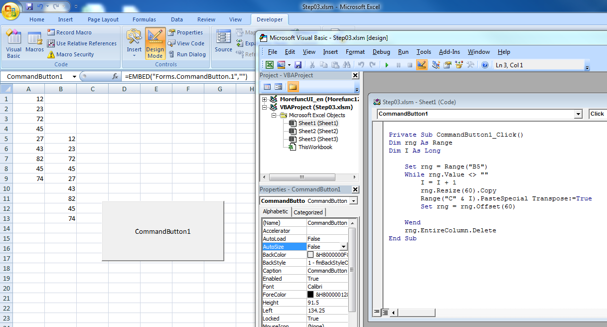
Code 0a: Snippet using the Copy method, and Paste method

Range("Sheet1!A2:A10").Select
    Selection.Copy

Range("Sheet2!B2").Select
    ActiveSheet.Paste

If instead, the user attempts to only use the Range objects directly, then the following code will return an error (Run-time error ‘438’, Object doesn’t support this property of method’) on the second statement.

Range("Sheet1!A2:A10").Copy

Range("Sheet2!B2").Paste    ' 

While Copy is a Method of the Range object, the Paste item is not. The VBE Object Browser lists only the following objects: Chart, Floor, Point, Series, SeriesCollection, Walls and Worksheet as having a member Paste method. Instead, the Range.PasteSpecial method is available as shown in the next section.

1.1 Workbook setup

Code 0b: Macro to the structure for the examples in this module

Sub SetUp()
Dim i As Integer

    Worksheets("Sheet1").Activate
    Names.Add Name:="Source", RefersTo:="=$A$2:$A$10"
    For i = 0 To 8
        Range("A2").Offset(i, 0) = 100 * (i + 1)
        Range("A2").Offset(i, 1) = 10 * (i + 1)
    Next i

    Worksheets("Sheet2").Activate
    Names.Add Name:="Target", RefersTo:="=$B$2"

End Sub

Openpyxl read multiple cells

We have the following data sheet:

Figure: Items

We read the data using a range operator.

read_cells2.py

#!/usr/bin/python

import openpyxl

book = openpyxl.load_workbook('items.xlsx')

sheet = book.active

cells = sheet

for c1, c2 in cells:
    print("{0:8} {1:8}".format(c1.value, c2.value))

In the example, we read data from two columns using a range operation.

cells = sheet

In this line, we read data from cells A1 — B6.

for c1, c2 in cells:
    print("{0:8} {1:8}".format(c1.value, c2.value))

The function is used for neat output of data
on the console.

$ ./read_cells2.py
Items    Quantity
coins          23
chairs          3
pencils         5
bottles         8
books          30

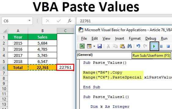
Вставить значения

Вставить значения — вставляет только «значение» ячейки. Если ячейка содержала формулу, функция «Вставить значения» вставит результат формулы.

Этот код скопирует и вставит значения для одной ячейки на том же листе:

12	Диапазон («A1»). КопироватьДиапазон («B1»). PasteSpecial Paste: = xlPasteValues

Копировать и вставлять значение на другой лист

В этом примере будут скопированы и вставлены значения для отдельных ячеек на разных листах.

12	Листы («Лист1»). Диапазон («А1»). КопироватьЛисты («Sheet2»). Range («B1»). PasteSpecial Paste: = xlPasteValues

Эти примеры будут копировать и вставлять значения для диапазонов ячеек:

Вставить значения и числовые форматы

При вставке значений будет вставлено только значение ячейки. Форматирование не вставляется, включая форматирование чисел.

Часто, когда вы вставляете значения, вы, вероятно, захотите также включить форматирование чисел, чтобы ваши значения оставались отформатированными. Давайте посмотрим на пример.

Здесь мы вставим значение ячейки, содержащей процент:

12	Таблицы («Sheet1»). Столбцы («D»). КопироватьТаблицы («Sheet2»). Столбцы («B»). PasteSpecial Paste: = xlPasteValues

Обратите внимание, как теряется форматирование процентного числа, и вместо него отображается неаккуратное десятичное значение. Вместо этого давайте использовать форматы вставки значений и чисел:

Вместо этого давайте использовать форматы вставки значений и чисел:

12	Таблицы («Sheet1»). Столбцы («D»). КопироватьЛисты («Sheet2»). Столбцы («B»). PasteSpecial Paste: = xlPasteValuesAndNumberFormats

Теперь вы можете видеть, что форматирование чисел также вставлено с сохранением процентного формата.

.Value вместо .Paste

Вместо вставки значений вы можете использовать свойство Value объекта Range:

Это установит значение ячейки A2 равным значению ячейки B2.

1	Диапазон («A2»). Значение = Диапазон («B2»). Значение

Вы также можете установить диапазон ячеек, равный значению одной ячейки:

1	Диапазон («A2: C5»). Значение = Диапазон («A1»). Значение

или диапазон ячеек, равный другому диапазону ячеек такого же размера:

1	Диапазон («B2: D4»). Значение = Диапазон («A1: C3»). Значение

Использование свойства Value требует меньше усилий. Кроме того, если вы хотите освоить Excel VBA, вы должны быть знакомы с работой со свойством ячеек «Значение».

Значение ячейки и свойство Value2

Технически лучше использовать свойство Value2 ячейки. Value2 немного быстрее (это имеет значение только при очень больших вычислениях), а свойство Value может дать вам усеченный результат, если ячейка отформатирована как валюта или дата. Однако более 99% кода, который я видел, использует .Value, а не .Value2. Я лично не использую .Value2, но вы должны знать, что он существует.

1	Диапазон («A2»). Значение2 = Диапазон («B2»). Значение2

Копировать Paste Builder

Мы создали «Copy Paste Code Builder», который упрощает создание кода VBA для копирования (или вырезания) и вставки ячеек. Строитель является частью нашей Надстройка VBA: AutoMacro.

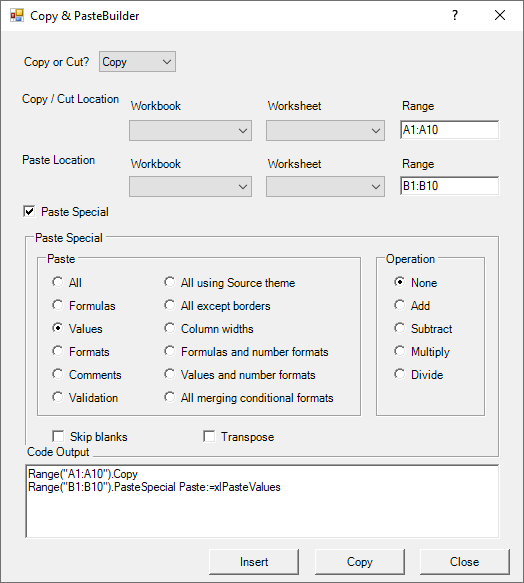
AutoMacro также содержит много других Генераторы кода, обширный Библиотека кодаи мощный Инструменты кодирования.

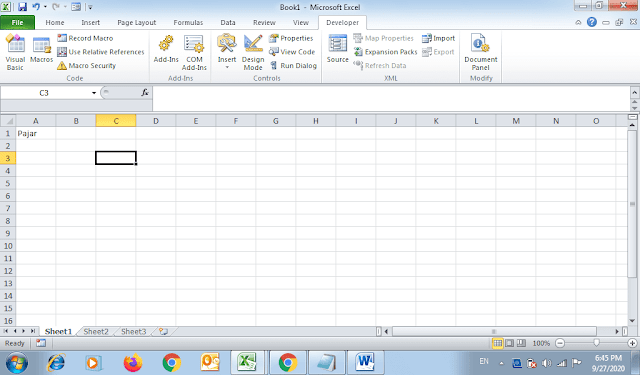
Use the Excel Screenshot Tool

Microsoft Excel, Word, and PowerPoint come with a built-in screenshot app. It allows you to take a screenshot of any other window except the current document on which you’re working.

The idea is to grab screenshots of other windows and include them in your active Excel workbook.

To use this method, you need to open two Excel workbooks. One is the source worksheet that contains your tables. The other is a blank Excel workbook where you’ll import the tables as images.

Click the screenshot tool on Excel

Find below a step-by-step guide to using the Excel screenshot tool:

1. Go to the blank Excel workbook.
2. Click the Screenshot button inside the Illustrations commands block of the Insert tab.
3. On the Available Windows context menu, choose the window that shows the Excel worksheet containing the table.

Click the screenshot tool on Excel

4. You should see a screenshot of the selected Excel worksheet along with the table.
5. Click the inserted image.
6. Then, click the Crop command button inside the Size block of the Picture Format tab.
7. You can now crop the image to only show the table using the cropping guides.
8. Click the Crop button again to finalize cropping.

You can follow the exact same steps in PowerPoint or Word to save an Excel table as an image in these apps.

This method is suitable to grab screenshots from Excel workbooks when you’re working on Excel, PowerPoint, or Word. You can import an image version of the target Excel table without needing any third-party tools.

Openpyxl read cell

In the following example, we read the previously written data from the
file.

read_cells.py

#!/usr/bin/python

import openpyxl

book = openpyxl.load_workbook('sample.xlsx')

sheet = book.active

a1 = sheet
a2 = sheet
a3 = sheet.cell(row=3, column=1)

print(a1.value)
print(a2.value)
print(a3.value)

The example loads an existing xlsx file and reads three cells.

book = openpyxl.load_workbook('sample.xlsx')

The file is opened with the method.

a1 = sheet
a2 = sheet
a3 = sheet.cell(row=3, column=1)

We read the contents of the A1, A2, and A3 cells. In the third line, we use the
method to get the value of A3 cell.

$ ./read_cells.py
56
43
10/26/16

Соединение макросов

Последовательность процесса выполнения операции ввода даты, порядковых номеров и замены формул значениями приведена на рисунке 6. Но прежде чем заставить макросы выполнять последовательно все записанные операции их необходимо соединить друг с другом.

Рис.6. Последовательность действий полного макроса РасходныйОрдер

• перенос написанных макросов Макрос2 , Макрос3 и Макрос4 в один макрос РасходныйОрдер в той последовательности, в которой они записывались;
• редактирование полученного макроса РасходныйОрдер и добавления процедур с целью последовательного выполнения операций показанных на рисунке 6;
• ввод примечаний.

Для соединения макросов в один примените метод копирования. Для этого в окне Редактора Visual Basic выделите область от конца последнего символа вверх кода VBA , включая первый встречающийся знак апострофа, как это показано на рисунке 7.

Рис.7. Выделение фрагмента макроса для копирования и вставки в другой макрос

После соединения всех макросов получился макрос, показанный на рисунке 8.

Рис.8. Макрос, полученный в результате соединения четырех макросов

Но данный макрос «работать» не будет, потому что он произведет вставку всех формул в одной и той же выделенной ячейке, которая перед выполнением макроса была активна.

Адресация ячеек в диапазоне

К ячейкам присвоенного диапазона можно обращаться по их индексам, а также по индексам строк и столбцов, на пересечении которых они находятся.

Индексация ячеек в присвоенном диапазоне осуществляется слева направо и сверху вниз, например, для диапазона размерностью 5х5:

1	2	3	4	5
6	7	8	9	10
11	12	13	14	15
16	17	18	19	20
21	22	23	24	25

Индексация строк и столбцов начинается с левой верхней ячейки. В диапазоне этого примера содержится 5 строк и 5 столбцов. На пересечении 2 строки и 4 столбца находится ячейка с индексом 9. Обратиться к ней можно так:

Обращаться в переменной диапазона можно не только к отдельным ячейкам, но и к части диапазона (поддиапазону), присвоенного переменной, например,

обращение к первой строке присвоенного диапазона размерностью 5х5:

и обращение к первому столбцу присвоенного диапазона размерностью 5х5: