Vba isnull function in excel

How do you show NULL in Excel?

Click File > Options > Advanced.
Under Display options for this worksheet, select a worksheet, and then do one of the following: To display zero (0) values in cells, select the Show a zero in cells that have zero value check box.

What does NULL mean in Excel?

NULL is nothing but nothing or blank in excel. Usually, when we are working in excel, we encounter many NULL or Blank cells. We can use the formula and find out whether the particular cell is blank (NULL) or not.

What is null error?

This error occurs when you’re passing on a null value. A null value means that there is actually no value in this variable. It’s not even a zero. String is the major case for this exception because other variables sometimes get a zero value, and hide this error. Arrays give out this error, when they’re empty.

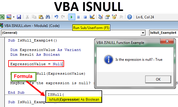
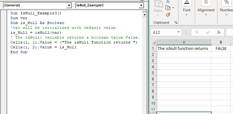
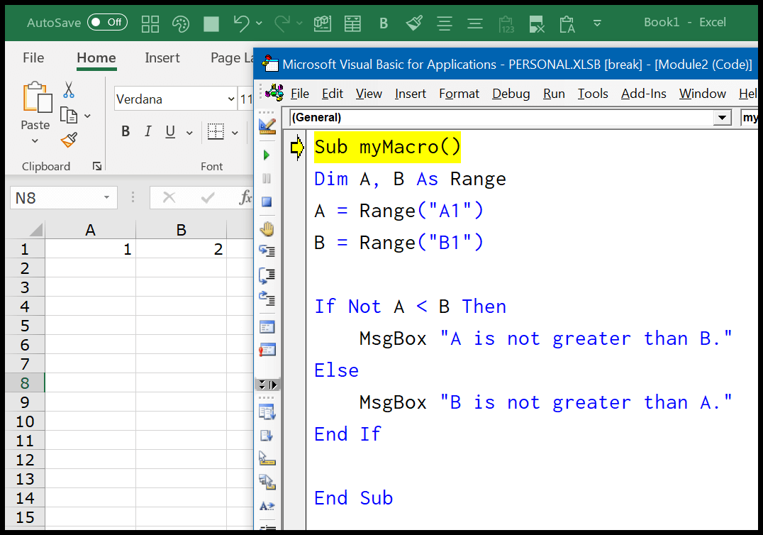
Is null VBA function?

ISNULL is a built-in function in VBA and is categorized as an Information function in VBA which returns the result in Boolean type i.e. either TRUE or FALSE. If the testing value is “NULL” then it returns TRUE or else it will return FALSE.

What is the value of null?

A null value indicates a lack of a value, which is not the same thing as a value of zero. For example, consider the question “How many books does Adam own?” The answer may be “zero” (we know that he owns none) or “null” (we do not know how many he owns).

How do you stop null in Excel?

How to remove blank cells in Excel

Select the range where you want to remove blanks.
Press F5 and click Special… .
In the Go To Special dialog box, select Blanks and click OK.
Right-click any of the selected blanks, and choose Delete… from the context menu:

What is ref in Excel?

The #REF! error shows when a formula refers to a cell that’s not valid . This happens most often when cells that were referenced by formulas get deleted, or pasted over.

How do I get a null error?

If you get this error because you’ve used a space character between ranges that don’t intersect, change the references so that ranges do intersect. For example, in the formula =CELL(“address”,(A1:A5 C1:C3)), the ranges A1:A5 and C1:C3 don’t intersect, and the formula returns the #NULL! error.

What does null value mean in Excel?

Null is an error value in a cell when an Excel cannot properly evaluate a worksheet formula or function.

How do you check if a range of cells is blank in Excel?

The ISBLANK function in Excel checks whether a cell is blank or not. Like other IS functions, it always returns a Boolean value as the result: TRUE if a cell is empty and FALSE if a cell is not empty.

Is null Excel function?

ISBLANK Function to Find NULL Value in Excel In excel, we have a built-in function called ISBLANK function, which can find the blank cells in the worksheet. Let’s look at the syntax of the ISBLANK function. If the cell is NULL, then it will return TRUE, or else it will return FALSE.

How do you check if multiple cells are blank in Excel?

The below formula can help you check if a range of cells is blank or not in Excel. Please do as follows. 1. Select a blank cell, enter formula =SUMPRODUCT(–(G1:K8<>””))=0 into the formula bar, and then press the Enter key.

How do you make a cell blank in Excel with no value?

To display zero (0) values as blank cells, uncheck the Show a zero in cells that have zero value check box….Display or hide zero values.

A	B
Formula	Description (Result)
=A2-A3	Second number subtracted from the first (0)
=IF(A2-A3=0,””,A2-A3)	Returns a blank cell when the value is zero (blank cell)

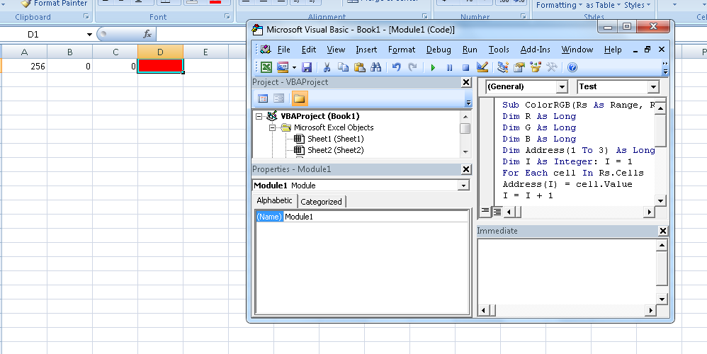
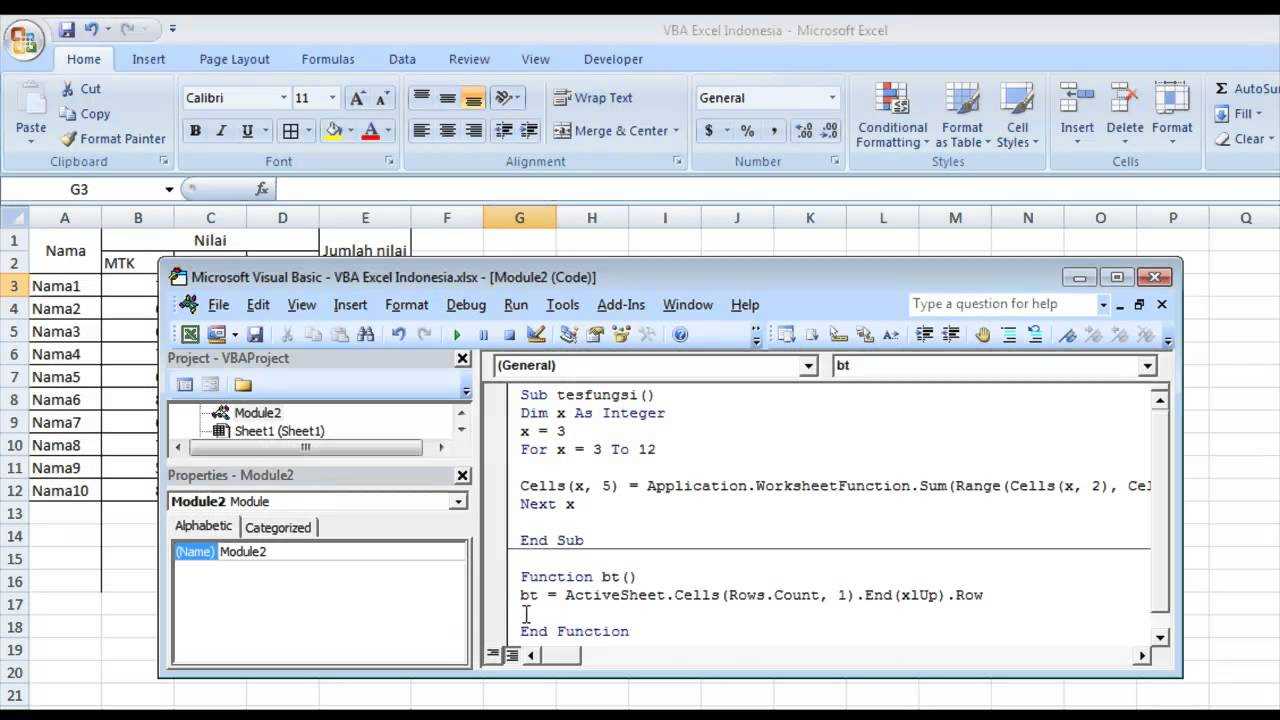
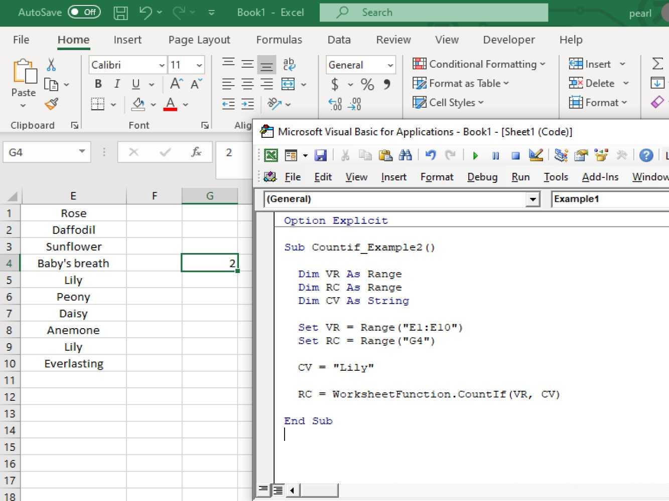
Catching Data Variation with IsNull

The other major source of Null values may fall out of the evaluation of built-in VBA functions or properties that are not producing expected results — hence the “invalid data” piece of the VBA IsNull function.

Using the same data set from above, let’s say you instruct employees to highlight any tentative details, such as the shipping method, with a different background color. To check whether any such highlights exist, you can write a simple one-liner to test for variation in cell background colors:

Conditional statements like are probably the most common way people use the VBA IsNull function.

Notice in this case you don’t have to assign the output to any variable at all and can simply feed the output of the property to the function.

Нулевой в Excel

NULL — это не что иное, как ничего или пустое значение в excel. Обычно, когда мы работаем в Excel, мы сталкиваемся со многими NULL или пустыми ячейками. Мы можем использовать формулу и выяснить, является ли конкретная ячейка пустой (NULL) или нет.

У нас есть несколько способов найти NULL-ячейки в Excel. В сегодняшней статье мы рассмотрим работу со значениями NULL в Excel.

Как определить, какая ячейка на самом деле пустая или пустая? Да, конечно, нам просто нужно посмотреть на конкретную ячейку и принять решение. Давайте откроем для себя множество методов поиска нулевых ячеек в Excel.

Функция ISBLANK для поиска значения NULL в Excel

В Excel у нас есть встроенная функция ISBLANK function, которая может находить пустые ячейки на листе. Давайте посмотрим на синтаксис функции ISBLANK.

Синтаксис прост и понятен. Значение не что иное, как ссылка на ячейку; мы проверяем, пусто оно или нет.

Поскольку ISBLANK — это логическая функция Excel, в результате она вернет TRUE или FALSE. Если ячейка ПУСТО (NULL), она вернет ИСТИНА, иначе она вернет ЛОЖЬ.

Заметка: ISBLANK будет рассматривать один пробел как один символ, и если ячейка имеет только значение пробела, то она будет распознаваться как непустая или непустая ячейка.

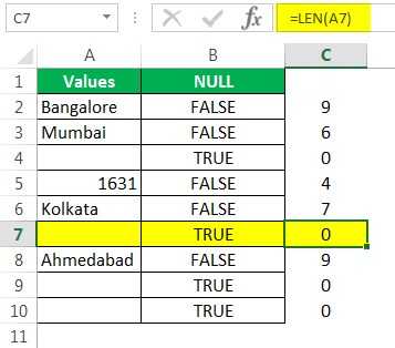
# 1 — Как найти NULL ячейки в Excel?

Предположим, у вас есть указанные ниже значения в файле Excel и вы хотите протестировать все пустые ячейки в диапазоне.

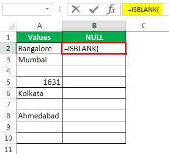
Выберите ячейку A2 в качестве аргумента. Поскольку есть только один аргумент, закройте скобку

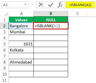
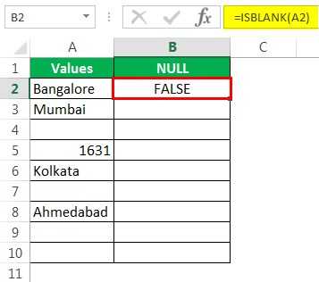
Мы получили результаты, но посмотрим на ячейку B7, хотя в ячейке A7 нет значения, формула все равно вернула результат как False, т.е. ненулевую ячейку.

Давайте применим функцию LEN в Excel, чтобы найти номер. символов в ячейке.

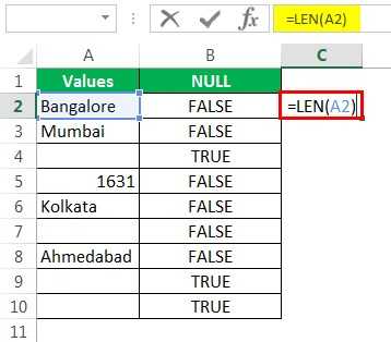
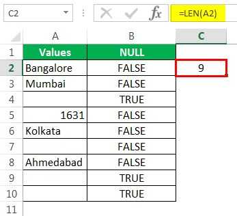
Функция LEN вернула номер символа в ячейке A7 как 1. Итак, в нем должен быть символ.

Теперь отредактируем ячейку. Итак, мы нашли здесь пробел; удалим пробел, чтобы формула показывала точные результаты.

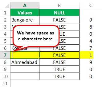
Я удалил пробел, и формула ISBLANK вернула результат как ИСТИНА, и даже функция LEN сообщает, что в ячейке A7 нулевые символы.

# 2 — Быстрый способ поиска NULL ячеек в Excel

Мы видели традиционный способ поиска нулевых ячеек с помощью формулы. Без использования функции ISBLANK мы можем найти нулевые ячейки.

После равенства sing выбирает ячейку A2 в качестве ссылки.

Теперь откройте еще один знак равенства после ссылки на ячейку.

Теперь упомяните открытые двойные кавычки и закрытые двойные кавычки. («»)

Знаки двойных кавычек («») указывают, что выбранная ячейка ПУСТО (NULL) или нет. Если выбранная ячейка — ПУСТО (NULL), тогда мы получим ИСТИНА, иначе мы получим ЛОЖЬ.

Мы видим, что в ячейке B7 мы получили результат «Истина». Это означает, что это пустая ячейка.

# 3 — Как заполнить наши собственные значения до NULL ячеек в Excel?

Мы видели, как найти NULL-ячейки на листе Excel. В нашей формуле в результате мы могли получить только ИСТИНА или ЛОЖЬ. Но мы также можем получить свои собственные значения для NULL ячеек.

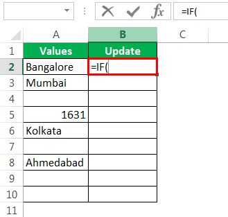
Шаг 2: Здесь нам нужно провести логический тест, то есть нам нужно проверить, является ли ячейка NULL или нет. Так что примените A2 = ””.

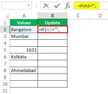
Шаг 3: Если логический тест — ИСТИНА (ИСТИНА означает, что ячейка НУЛЯ), нам нужен результат как «Значения не найдены».

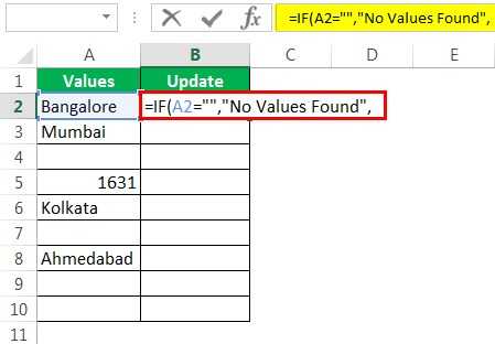
Шаг 4: Если логический тест — ЛОЖЬ (ЛОЖЬ означает, что ячейка содержит значения), то нам нужно то же значение ячейки.

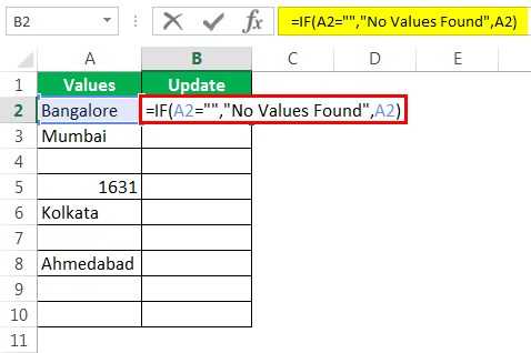
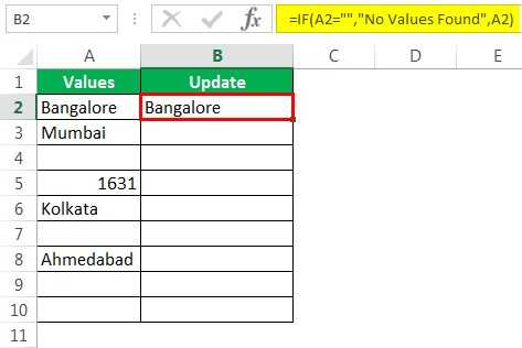
Шаг 5: Перетащите формулу в оставшиеся ячейки.

Итак, у нас есть своя ценность Значения не найдены для всех ячеек NULL.

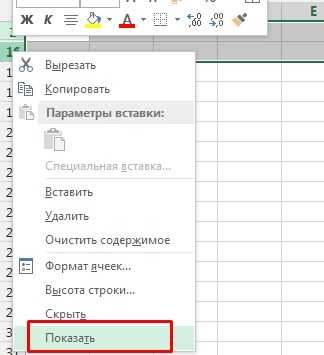
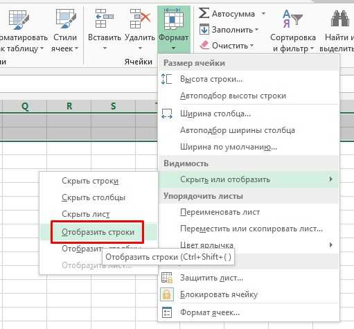
Сразу нужно сказать, что выбор варианта включения отображения скрытых элементов в первую очередь зависит от того, каким образом они были скрыты. Зачастую эти способы используют совершенно разную технологию. Существуют такие варианты скрыть содержимое листа:

Conclusion:

Hope after reading this article it is clear to you how these errors arise and the fixes given will help you to resolve #REF, #NUM, #NAME, #N/A, #VALUE, #NULL, #DIV/0, ##### error.

Make sure to follow the fixes carefully to avoid further errors. If in case you are having any queries you can tell us in the below comment I assure you to fix it soon.

Priyanka Sahu

Priyanka is a content marketing expert. She writes tech blogs and has expertise in MS Office, Excel, and other tech subjects. Her distinctive art of presenting tech information in the easy-to-understand language is very impressive. When not writing, she loves unplanned travels.

Когда использовать возвратить null в Excel

Функция Возвратить null в Excel используется в контексте ошибок или отсутствия данных. Когда некоторые ячейки не содержат значений или возвращает ошибку, возвратить null позволяет явно указать отсутствие данных или ошибку.

Если, например, у вас есть формула, которая выполняет вычисление на основе значений в других ячейках, и одна или несколько этих ячеек пустые или содержат ошибку, вы можете использовать функцию Возвратить null для отображения отсутствия данных для этой формулы.

Возвратить null также полезно, когда вы хотите обозначить отсутствие значения или ошибку в других пользовательских функциях или макросах в Excel. Это может быть особенно полезно, если вам нужно отдельно обработать случай отсутствия данных или ошибки в вашем коде.

Использование Возвратить null позволяет более явно выражать и обрабатывать состояние отсутствия данных или ошибки в Excel, что может помочь вам в работе с данными и обеспечить более точную обработку ошибок в вашей таблице.

Hide Zero Value in Cells using Conditional Formatting

While the above method is the most convenient one, it doesn’t allow you to hide zeros only in a specific range (rather it hides zero values in the entire worksheet).

In case you only want to hide zeros for a specific dataset (or multiple datasets), you can use conditional formatting.

With conditional formatting, you can apply a specific format based on the value in the cells. So, if the value in some cells is 0, you can simply program conditional formatting to hide it (or even highlight it if you want).

Suppose you have a dataset as shown below and you want to hide zeros in the cells.

Below are the steps to hide zeros in Excel using conditional formatting:

Select the dataset
Click the ‘Home’ tab
In the ‘Styles’ group, click on ‘Conditional Formatting’.
Place the cursor over the ‘Highlight Cells Rules’ options and in the options that show up, click on the ‘Equal to’ option.
In the ‘Equal To’ dialog box, enter ‘0’ in the left field.
Select the Format drop-down and click on ‘Custom Format’.
In the ‘Format Cells’ dialog box, select the ‘Font’ tab.
From the Color drop-down, choose the white color.
Click OK.
Click OK.

The above steps change the font color of the cells that have the zeros to white, which make these cells look blank.

This workaround works only when you have a white background in your worksheet. In case there is any other background-color in the cells, the white color may still keep the zeros visible.

In case you want to truly hide the zeros in the cells, where the cells look blank no matter what background color is given to the cells, you can use the steps below.

Select the dataset
Click the ‘Home’ tab
In the ‘Styles’ group, click on ‘Conditional Formatting’.
Place the cursor over the ‘Highlight Cells Rules’ options and in the options that show up, click on the ‘Equal to’ option.
In the ‘Equal To’ dialog box, enter 0 in the left field.
Select the Format drop-down and click on Custom Format.
In the ‘Format Cells’ dialog box, select the ‘Number’ tab and click on the ‘Custom’ option in the left pane.
In the Custom format option, enter the following in the Type field: ;;; (three semi-colons without space)
Click OK.
Click OK.

The above steps change the custom formatting of cells that have the value 0.

When you use three semi-colons as the format, it hides everything in the cell (be it numeric or text). And since this format is applied only to those cells which have the value 0 in it, it only hides the zeros and not the rest of the dataset.

You can also use this method to highlight these cells in a different color (such as red or yellow). To do this, just add another step (after Step where you need to select the Fill tab in the ‘Format cells’ dialog box and then select the color in which you want to highlight the cells.

Both the methods covered above also work when 0 is a result of a formula in a cell.

Note: Both the method covered in this section only hide the zero values. It doesn’t remove these zeros. This means that in case you use these cells in calculations, all the zeros will be used as well.

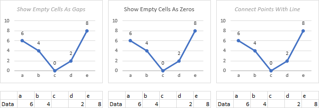
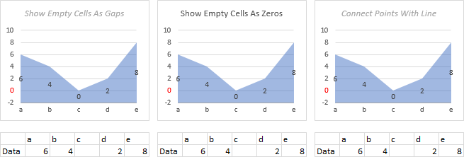
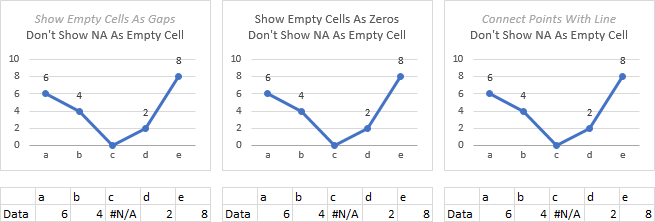
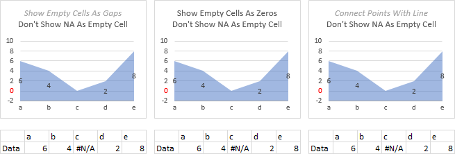
Excruciating Detail: Plotting Blanks and #N/A Values in Stacked Excel Charts

This section was moved to the end, because it seemed to present too much information at once, and confuse more than clarify. But now that you’ve seen the comparisons above, it might be safe to continue.

Plot Empty Cells in Stacked Excel Charts

These settings work differently in stacked charts. Excel’s rationale is that you can’t plot a gap, because the point stacked on top of the gap might have a value, and it needs something for it to be stacked on. If you are trying to plot an empty cell as a gap, and it isn’t working, make sure you aren’t using a stacked chart type. I should note that Excel does not apply this rationale consistently.

One of the most confusing chart types is a stacked line. People choose it when selecting a chart type, not realizing that each series’ values are plotted on top of previous values. (It’s much easier to notice stacked series and comprehend the data in a stacked column or area chart).

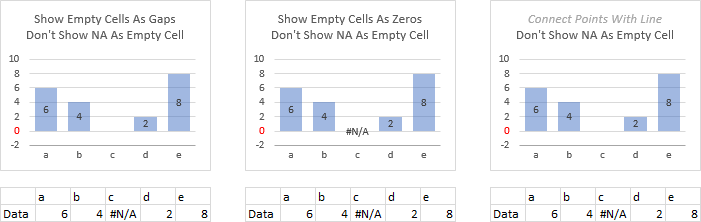
This is how Excel plots a blank cell in a stacked line chart (it has only one series, but it’s still a stacked line chart). The only option you can select is Show as Zeros (though you can apply the other settings through the roundabout means described earlier), and what you always get is a point at zero.

In a stacked column chart, you have both the As Gap and As Zero options available. As Zero results in a zero-height data point (i.e., bar), which we can see because of the data label; As Gaps seems to lack this data point, in conflict with Excel’s apparent decision that it needs a zero point to stack subsequent point on. The disabled Interpolate setting reverts to As Gaps. Note that in the stacked column chart, the bars start at zero, not at the axis.

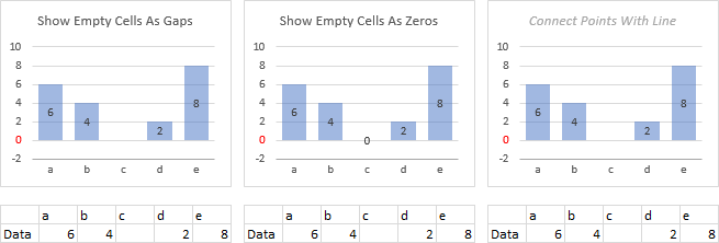
When you add Series Lines to the stacked column chart (please don’t use these confusing bits of clutter), the series lines connect the bars on either side of the gap (left and right), and connect with the zero-height bar when plotted As Zero (center).

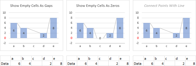
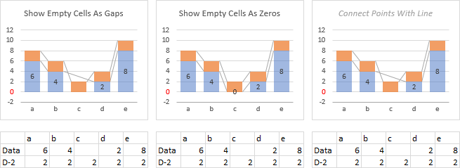
If we stack another series of bars atop our series with the blank value, we see two things. The second bar has no problem stacking on the place a missing bar would be, and the series lines show an interesting crossing pattern.

Like the line chart, the stacked area chart only has the As Zeros option available, and you can see the zero-value point where the blank cell goes.

Plot #N/A in Stacked Excel Charts

In a stacked line chart, #N/A is plotted as zero, since you need a point on which to stack other series. The #N/A zero points have markers but no data labels.

In a stacked column chart, the behavior is similar to the plotting of blank cells. Even though the #N/A is supposedly not treated as a blank, there are different behaviors based on the Show Empty Cells setting: As Gaps results in no apparent point, because there is no data label, while the As Zeros setting apparently plots a bar 0 units high, evidenced by the #N/A label. Unlike in the unstacked column charts above, bars start not at the X-axis but at zero, so we can’t actually see the zero-height bar. Connect Points With Line is undefined as before but reverts to the As Gaps behavior.

When we add series lines, we see further evidence for the data point in the As Zeros case: the series lines drop to the top of the zero-height bar in the center.

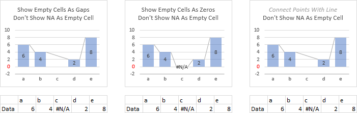
In an area chart, only the As Zeros case is enabled, and whatever the setting, the appearance of the chart is the same: the #N/A value results in a point at zero, with no data label.

#ССЫЛКА! в ячейке

Иногда это может немного сложно понять, но Excel обычно отображает #ССЫЛКА! в тех случаях, когда формула ссылается на недопустимую ячейку. Вот краткое изложение того, откуда обычно возникает эта ошибка:

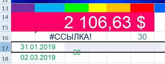
Что такое ошибка #ССЫЛКА! в Excel?

#ССЫЛКА! появляется, если вы используете формулу, которая ссылается на несуществующую ячейку. Если вы удалите из таблицы ячейку, столбец или строку, и создадите формулу, включающую имя ячейки, которая была удалена, Excel вернет ошибку #ССЫЛКА! в той ячейке, которая содержит эту формулу.

Теперь, что на самом деле означает эта ошибка? Вы могли случайно удалить или вставить данные поверх ячейки, используемой формулой. Например, ячейка B16 содержит формулу =A14/F16/F17.

Если удалить строку 17, как это часто случается у пользователей (не именно 17-ю строку, но… вы меня понимаете!) мы увидим эту ошибку.

Здесь важно отметить, что не данные из ячейки удаляются, но сама строка или столбец

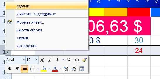
Как исправить #ССЫЛКА! в Excel?

Прежде чем вставлять набор ячеек, убедитесь, что нет формул, которые ссылаются на удаляемые ячейки

Кроме того, при удалении строк, столбцов, важно дважды проверить, какие формулы в них используются

Совет для профессионалов
Если вы случайно удалили несколько ячеек, вы можете восстановить их нажатием кнопки «Отменить» на панели быстрого доступа. Сочетание клавиш CTRL + Z для Windows и Command + Z для Mac, также позволяет отменить последние внесенные изменения.

Примеры использования функции NULL в Excel

Вот несколько примеров использования функции NULL:

Пример 1:

Предположим, у вас есть столбец, содержащий имена сотрудников, и вы хотите проверить, есть ли в этом столбце пустые ячейки. Для этого вы можете использовать функцию NULL следующим образом:

=ЕСЛИ(НЕ(NULL(A1)); "Ячейка не пуста"; "Ячейка пуста")

Функция NULL(A1) вернет истинное значение, если ячейка A1 не пуста, и ложное значение, если ячейка пуста. Таким образом, в результате выполнения формулы вы увидите «Ячейка не пуста» или «Ячейка пуста» в зависимости от содержимого ячейки A1.

Пример 2:

Предположим, у вас есть два столбца, A и B, содержащие числовые значения, и вы хотите найти среднее только для непустых ячеек. Для этого вы можете использовать функцию NULL совместно с функцией СРЗНАЧ:

=СРЗНАЧ(NULL(A1:B10); "")

Функция NULL(A1:B10) вернет массив всех значений в диапазоне A1:B10, в которых ячейки не являются пустыми. Затем функция СРЗНАЧ вычислит среднее значение только для непустых ячеек. Если в диапазоне нет непустых ячеек, то функция СРЗНАЧ вернет пустую строку.

Пример 3:

Предположим, у вас есть столбец с датами и вы хотите отфильтровать только строки, где ячейки содержат конкретную дату. Для этого вы можете использовать функцию NULL следующим образом:

=ЕСЛИ(NULL(A1) = ДАТА(2020; 1; 1); "Ячейка содержит указанную дату"; "Ячейка не содержит указанную дату")

Функция NULL(A1) будет возвращать ложное значение для пустых ячеек и истинное значение, если ячейка A1 содержит конкретную дату (в данном случае, 1 января 2020 года). Таким образом, вы получите результат «Ячейка содержит указанную дату» или «Ячейка не содержит указанную дату» в зависимости от содержимого ячейки A1.

Вышеуказанные примеры показывают лишь некоторые из возможных способов использования функции NULL в Excel. Но в общем случае, функция NULL позволяет удобно работать с пустыми значениями в ячейках и упрощает выполнение различных операций и анализ данных.

Show Zero as Blank with Office Scripts

VBA isn’t the only way to automate things in Excel. You can also use Office Scripts if you’re using Excel online with a Microsoft 365 business plan.

Open your Excel workbook in the web browser and go to the Automate tab then select the New Script option.

This will open the Code Editor on the right side of the workbook. You can then copy and paste the above code into the Code Editor and press the Save script button.

This code will loop through the selected range and clear the content of any cell that contains a zero.

Select the range with zeros and press the Run button in the Code Editor and your zeros will be removed leaving you with blank cells in their place.

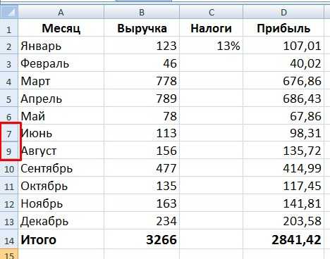
ЕСЛИОШИБКА в формулах массива

Как вы, наверное, знаете, формулы массива в Excel предназначены для выполнения нескольких вычислений внутри одной формулы. Если вы в аргументе значение функции ЕСЛИОШИБКА укажете формулу или выражение, которое возвращает массив, она также обработает и вернет массив значений для каждой ячейки в указанном диапазоне. Пример ниже поможет пояснить это.

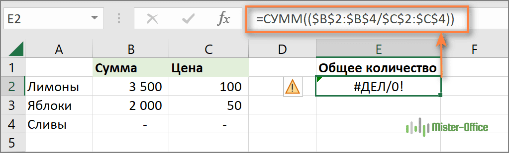
Допустим, у вас есть Сумма в столбце B и Цена в столбце C, и вы хотите вычислить Количество. Это можно сделать с помощью следующей формулы массива, которая делит каждую ячейку в диапазоне B2:B4 на соответствующую ячейку в диапазоне C2:C4, а затем суммирует результаты:

=СУММ(($B$2:$B$4/$C$2:$C$4))

Формула работает нормально, пока в диапазоне делителей нет нулей или пустых ячеек. Если есть хотя бы одно значение 0 или пустая строка, то возвращается ошибка: #ДЕЛ/0! Из-за одной некорректной позиции мы не можем получить итоговый результат.

Чтобы исправить эту ситуацию, просто вложите деление внутрь формулы ЕСЛИОШИБКА:

Результат вы видите на скриншоте ниже:

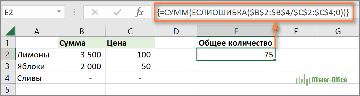
Что делает эта формула? Делит значение в столбце B на значение в столбце C в каждой строке (3500/100, 2000/50 и 0/0) и возвращает массив результатов {35; 40; #ДЕЛ/0!}. Функция ЕСЛИОШИБКА перехватывает все ошибки #ДЕЛ/0! и заменяет их нулями. Затем функция СУММ суммирует значения в итоговом массиве {35; 40; 0} и выводит окончательный результат (35+40=75).

Примечание. Помните, что ввод формулы массива должен быть завершен нажатием комбинации Ctrl + Shift + Enter (если у вас не Office365 или Excel2021 – они понимают формулы массива без дополнительных телодвижений).

Какие выгоды и преимущества имеет функция NULL в Excel

Функция NULL в Excel предоставляет ряд выгод и преимуществ, которые помогают пользователю управлять данными и выполнить различные операции. Ниже перечислены основные выгоды и преимущества функции NULL:

Удобство обработки пустых значений: Функция NULL позволяет определить ячейки с пустыми значениями и использовать их для обработки данных. Она предоставляет пользователю возможность легко определить и заменить пустые значения или применить к ним определенные операции.
Гибкость в работе с данными: Функция NULL позволяет использовать различные операции с ячейками, содержащими пустые значения. Это позволяет пользователю заменять, фильтровать или анализировать такие значения в соответствии с требуемыми условиями.
Управление ошибками: Функция NULL помогает пользователю контролировать ошибки, возникающие при работе с данными. Она позволяет избежать проблем, связанных с операциями, выполняемыми над пустыми значениями, и предоставляет возможность обрабатывать такие ошибки.
Моделирование отсутствующих данных: Функция NULL может быть использована для моделирования отсутствующих данных. Используя пустые значения, пользователь может создать и анализировать различные сценарии, связанные с отсутствием определенных данных.
Улучшенная читаемость и понимание данных: Функция NULL позволяет пользователям более точно представлять данные, особенно если они содержат пустые значения. Это помогает в лучшем понимании и анализе данных.
Удобство в работе с функциями и формулами: Функция NULL облегчает работу с функциями и формулами, особенно при использовании операций, требующих обработки пустых значений. Она предоставляет пользователю возможность гибкого управления данными и условиями в функциях.

Использование функции NULL в Excel может значительно упростить работу с данными и помочь в анализе и обработке информации. Она предоставляет пользователю широкий спектр возможностей и позволяет эффективно управлять данными, улучшая процесс принятия решений.

How do you NULL values in Excel?

ISBLANK Function to Find NULL Value in Excel In excel, we have a built-in function called ISBLANK function, which can find the blank cells in the worksheet. Let’s look at the syntax of the ISBLANK function. It returns the output “true” if the cell is empty (blank) or “false” if the cell is not empty.

How do I check if a value is null in Excel?

Excel ISBLANK Function

Summary. The Excel ISBLANK function returns TRUE when a cell is empty, and FALSE when a cell is not empty. For example, if A1 contains “apple”, ISBLANK(A1) returns FALSE.
Test if a cell is empty.
A logical value (TRUE or FALSE)
=ISBLANK (value)
value – The value to check.

Why does excel not show null values?

Click File > Options > Advanced. Under Display options for this worksheet, select a worksheet, and then do one of the following: To display zero (0) values in cells, check the Show a zero in cells that have zero value check box.

How do I filter null values in Excel?

Use a simple filter to remove blank rows in Excel

Select all columns that hold your data range.
Go to Ribbon > Data tab > Sort & Filter Group > Filter.
Move across the columns. Click the Filter dropdown for each column. Uncheck Select All then check Blanks for rows that have only some blank cells.

How do you indicate a blank cell in Excel?

We can use the ISBLANK coupled with conditional formatting. For example, suppose we want to highlight the blank cells in the range A2:F9, we select the range and use a conditional formatting rule with the following formula: =ISBLANK(A2:F9).

How do I convert 0 to blank in Excel?

Use Excel’s Find/Replace Function to Replace Zeros

Open your worksheet and either 1) select the data range to be changed or 2) select a single cell to change the entire worksheet.
Choose Find/Replace (CTRL-H).
Use 0 for Find what and leave the Replace with field blank (see below).

How do I show blanks in Excel instead of 0?

It’s very simple:

Select the cells that are supposed to return blanks (instead of zeros).
Click on the arrow under the “Return Blanks” button on the Professor Excel ribbon and then on either. Return blanks for zeros and blanks or. Return zeros for zeros and blanks for blanks.

How do I filter null value?

Filtering on your formula Or you can filter by left-clicking on a {blank} value in your search result table, then right-clicking and selecting Show only “{Blank}”.

How do you filter null?

The most common filter syntax to filter out nulls is simply “-NULL” . This works for most data types that aren’t numbers, such as strings, dates, etc.

How do I exclude a value from a list in Excel?

Please do as follows.

Select a blank cell which is adjacent to the first cell of the list you want to remove, then enter formula =COUNTIF($D$2:$D$6,A2) into the Formula Bar, and then press the Enter key.
Keep selecting the result cell, drag the Fill Handle down until it reaching the last cell of the list.

How do you calculate only if cell is not blank in Excel?

How to Calculate Only If Cell is Not Blank in Excel

=IF(AND(B3<>””,B2<>””),B2-B3,””) In this case, if any of the cells is blank, AND function returns false.
=IF(OR(ISBLANK(B3),ISBLANK(B2)),””,B2-B3) It does the same “if not blank then calculate” thing as above.
=IF(COUNTBLANK(B2:H2),””,SUM(B2:H2))

What is the opposite of Isblank in Excel?

The Excel NOT function returns the opposite of a given logical or Boolean value. When given TRUE, NOT returns FALSE. When given FALSE, NOT returns TRUE.

Is not function in Excel?

The NOT function is an Excel Logical function. The function helps check if one value is not equal to another. If we give TRUE, it will return FALSE and when given FALSE, it will return TRUE. So, basically, it will always return a reverse logical value.

Why is excel showing formula not result?

The reason for Excel showing formula not result. The reason this happens is because the cells which contain the formula have been formatted as text. You may have explicitly formatted them as text but more often it is a download or import from another system and the system has made all cells text.

Excel Formula Error #DIV/0!

This #DIV/0 error message appears when you are asking Excel to divide a formula by Zero or an empty cell. Well, you can’t perform this task in you are doing division by hand, or on a calculator, then how it is possible in Excel.

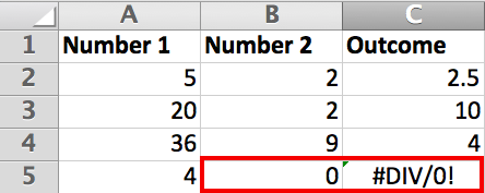
What Does #DIV/0! Mean In Excel?

The #DIV/0! error appears when any formula tries to get divided by zero. Excel #DIV/0! error gives a clear indication that something unexpected or some data is missing in Excel spreadsheet.

Generally this error encounters when data is entered Excel cell but it’s not complete. Suppose, worksheet cell’s is empty because of no data is present in it.

Reasons Behind Getting #DIV/0! Error In Excel

When the formula tries to segregate by zero, then the #DIV/0! error occurs. Other reasons are as follows:

the denominator or divisor in division operation equal to zero – either unambiguously – like =A5 / 0– or as a result of a subsequent calculation that has zero for the outcome;
a cell referencing formula that’s blank.

How To Remove #Div/0 In Excel?

Well, this is not a big issue and can be resolved easily. All you need to change the value of the cell to the value that is not equal to 0 or else inserts a value if your cell was blank.

Verify that you have accurate data in cells referenced within the formula.
Confirm whether data is into correct cells or not.
Ensure that the formula uses correct cell reference.