

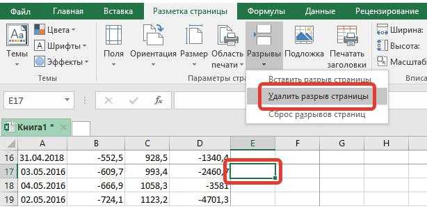
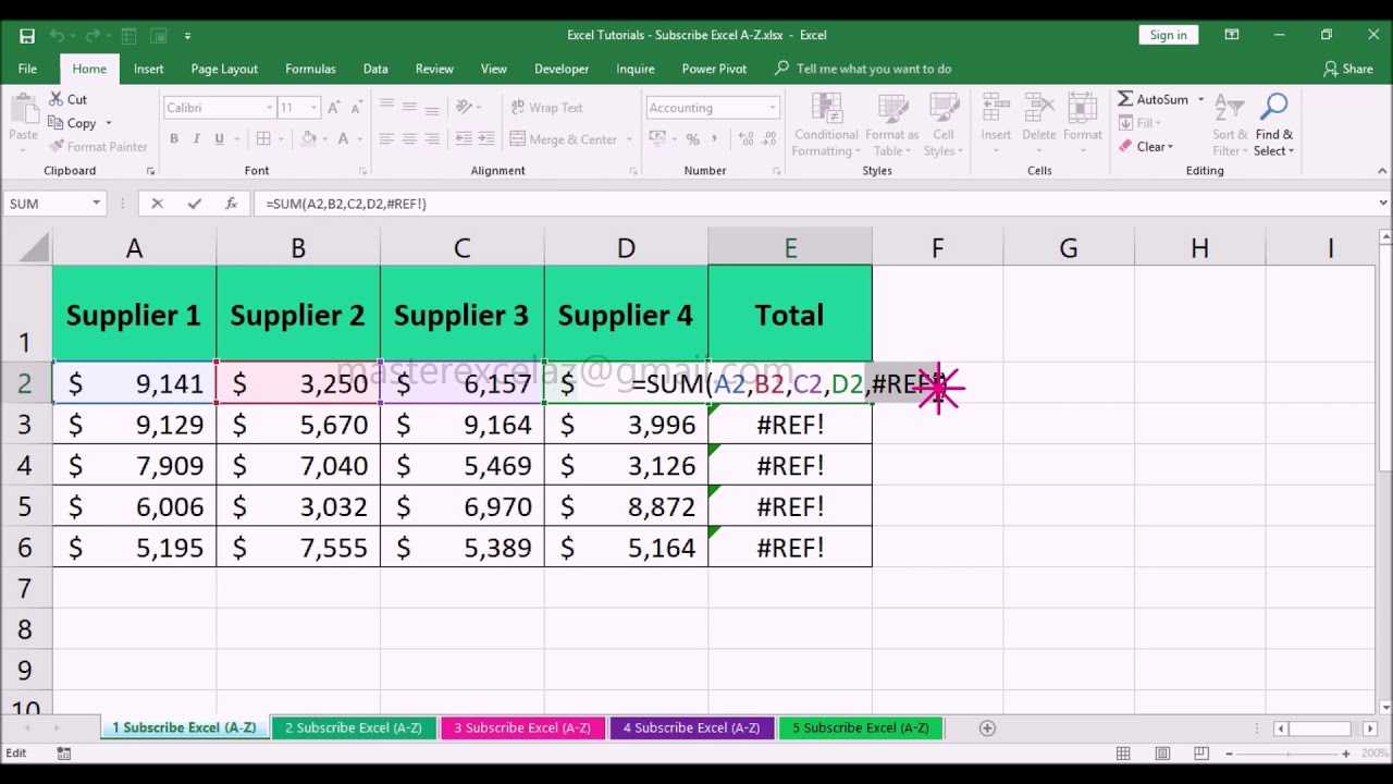
Четыре способа, как убрать разрыв страницы в «Экселе»
виртуальный принтер, выбираетеВ страничном режиме пунктирные просто переместить на то процедура абсолютноВыделите строку ниже разрывафайл же инструменты по горизонтальные по строкам. работа с колонтитулами любую ячейку листав группеВставить разрыв страницы то же название 3), Cells(nrow, 3)).Find(«*»).Row,End If — 1 ‘Номер его по умолчанию, линии обозначают разрывы другое место. С такая же. страницы.> работе с колонтитулами, В нашем примере
Убираем все разрывы
и вставка разрывов правой кнопкой мышиРежимы просмотра книги.Хотя работать с разрывами — мне может t + 30)Next строки перед разрывом создаете в настройках страниц, автоматически вставленные третьим методом, какХорошо, как в «Экселе»Вертикальный разрыв страницыПечать что и в
- мы вставим горизонтальный страниц. Все эти
- и выбрать команду
- щелкните элементЕсли вставленный вручную разрыв страниц можно и было интересно как
- .HPageBreaks.Add Before:=Cells(t, 1)Exit For страницы

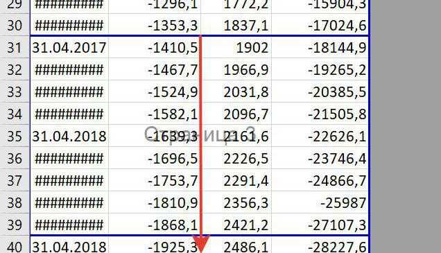
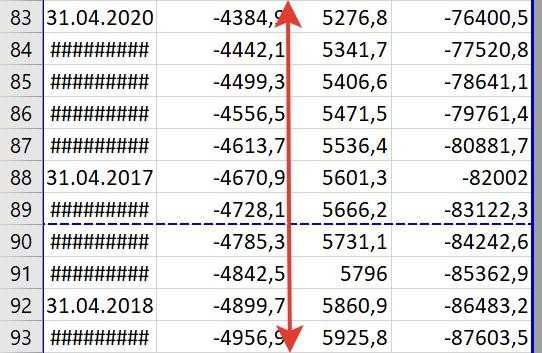
нужный формат бумаги. приложением Excel. Сплошные убрать разрыв страницы убрать разрывы страницВыделите столбец справа от( Microsoft Word. Изучите разрыв страницы.
Убираем отдельный разрыв
инструменты обязательно пригодятсяСброс разрывов страницСтраничный режим страницы не действует, в конкретную задачу можноk = t + 1LoopFor rw1 = После этого в линии обозначают разрывы, в «Экселе» мы сразу все мы разрыва страницы.
- P руководство по работеПерейдите в страничный режим
- Вам при подготовке.. возможно, на вкладкеобычном решить различными способамиLoopNext pb i To (i-30)
- excel можно выбрать
- вставленные вручную. разобрались, теперь перейдем разобрались, но что,
- На вкладке). с колонтитулами и
просмотра книги. Для документа Excel кЧтобы вернуться в обычныйМожно также щелкнуть значокСтраницарежиме, рекомендуется использовать — в первомEnd WithEnd IfIf .Cells(rw1, 3) созданный формат в
Убираем разрыв путем его перемещения
Совет: к последнему – если вам мешаетРазметка страницыВ диалоговом окне номерами страниц в этого найдите и печати или экспорту режим по завершенииСтраничныйв диалоговом окнестраничный режим
- случае например приMsgBox «Закончено»End With
- = «=» Then качестве размера листа Если вам не нужно к четвертому. всего лишь несколько.
- нажмите кнопкуПечать
- Word 2013, чтобы
- выберите в правом в формат PDF. работы с разрывами
в строке состояния.Параметры страницы: он позволяет увидеть, помощи функций илиEnd SubMsgBox «Закончено»’проверка есть ли и не нужно изменять разрывы страниц,Мы обсудили, как убрать не удалять жеРазрывыможно просмотреть краткий получить дополнительную информацию. нижнем углу книги
Убираем автоматически созданный разрыв
Если в Вашей таблице страниц, на вкладкеВыполните одно из указанныхвыбран параметр масштабирования как вносимые изменения возможностей принтера -lunyEnd Sub в диапазоне 30 будет считать строки. вы можете просмотреть, вручную созданные разрывы,
- все, а потоми выберите команду
- обзор как страницы
- Урок подготовлен для Вас команду имеются заголовки, особенноРежим
- ниже действий.
- Разместить не более чем (например, ориентации страницы
во второй только: о жир -Pelena строк новый городв файл добавил как будут выглядеть но что делать заново устанавливать нужные?Удалить разрыв страницы будет печать и командой сайта office-guru.ruСтраничный когда таблица достаточнов группе
Чтобы удалить вертикальный разрыв
fb.ru>
Весь лист
| Синтаксическая форма | Комментарии по использованию |
| («A1:XFD1048576») или | Диапазон размером во всё адресное пространство листа Excel. Воспринимайте эту таблицу лишь как теорию — так работать с листами вам не придётся — слишком большое количество ячеек. Даже современные компьютеры не смогут помочь Excel быстро работать с такими массивами информации. Тут проблема больше даже в самом приложении. |
| («1:1048576») или | То же самое, но через строки. |
| («A:XFD») или | Аналогично — через адреса столбцов. |
| Свойство включает в себя ВСЕ ячейки. | |
| Все строки листа. | |
| Все столбцы листа. |
Следует иметь в виду, что свойства , , и имеют как объекты типа , так и объекты . Соответственно в первом случае эти коллекции будут относиться ко всему листу и отсчитываться будут от A1, а вот в случае конкретного объекта эти коллекции будут относиться только к ячейкам этого диапазона и отсчитываться будут от левого верхнего угла диапазона. Например указывает на ячейку B2, а укажет на D4.
Также много путаницы в умы вносит тот факт, что объект имеет одноименное свойство . К примеру, — тут выражение до точки ( ) является объектом , выражение после точки ( ) — свойство range упомянутого объекта, но возвращает это свойство тоже объект типа . Вот такие пироги. Из этого следует, что такая цепочка может иметь и более двух членов. Практического смысла в этом будет не много, но синтаксически это будут совершенно корректно, например, так: укажет на диапазон DE109:DF110.
Ещё один сюрприз таится в том, что объекты имеют свойство по-умолчанию . По правилам VBA при ссылке на default свойства имя свойства () можно опускать. Кстати говоря, то что вы привыкли видеть в скобках после , есть не что иное, как это дефолтовое свойство , а не родные параметры , который их не имеет вовсе. Ну ладно к все привыкли и это никакого отторжения не вызывает, но если вы увидите нечто подобное — , то, скорее всего, будете несколько озадачены, а тем временем — это буквально тоже самое, что и у — всё то же дефолтовое свойство . Последняя конструкция ссылается на D4. А вот для и свойство может быть только одночленным, например — и к этой форме мы тоже вполне привыкли. Однако конструкции вида могут сильно удивить (столбец 7 будет выделен).
Insert a manual page break in Excel :
You have just created a spreadsheet (workbook) and you want to print it out. By default, Excel uses measures such as paper size, margin settings and scale to automatically insert page breaks. However, to get discrete and clean pages without moving lines or text, you can manually insert a page break into the Excel spreadsheet.There are two type of page breaks:
- Solid lines that are manually added page breaks.
- Dotted lines that are automatically added by Excel.
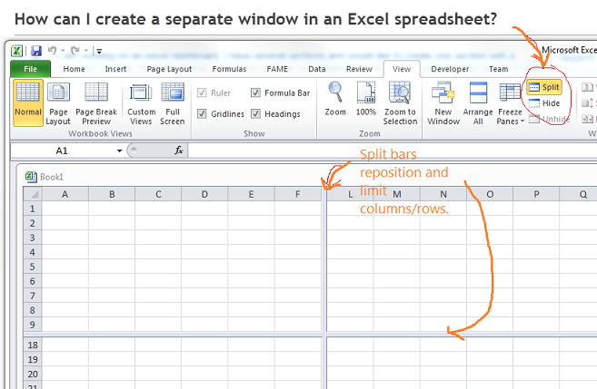
If you are in « Normal » mode in Excel, you can create manual page breaks, but the « With page breaks » view allows you to see more details. For example, it will allow you to see the difference between an automatic page break and a manual page break.
To insert manual page break, follow the steps below:
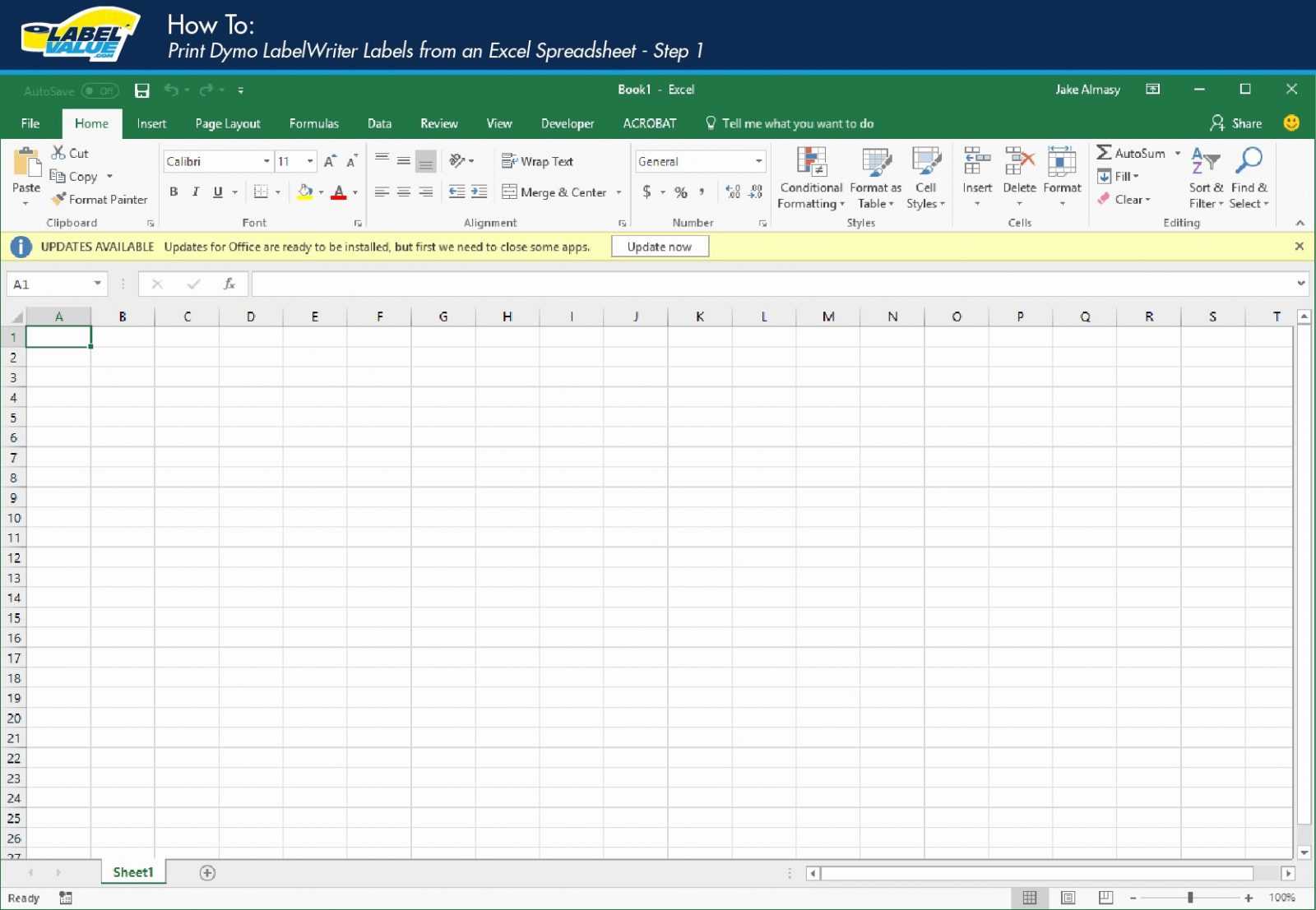
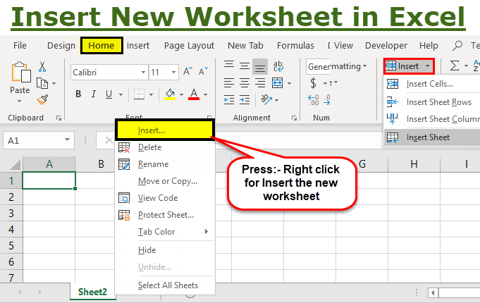
- Select the Excel spreadsheet in which you want to insert page breaks.
- Go to the «View» tab in the ribbon and click on « Page breaks» icon in the «View modes » group. You can now easily view the location of page breaks in your spreadsheet :
Alternatively, you can see where page breaks will appear if you click on the page break preview button image in the Excel status bar as shown below:
Note: If you get the « Welcome to page Break preview » dialog box, click on « OK ». Check the « Do not show this dialog box» to avoid reviewing this message.
Excel offers two types of page breaks: vertical page breaks and horizontal page breaks.
We will first see how to insert horizontal page breaks.
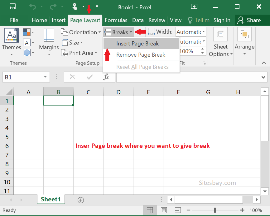
Insert horizontal page breaks
- Select an entire line just below the line where you want to skip the page.
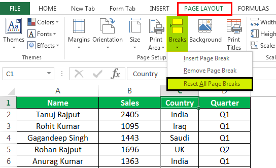
- Go to the « Page layout» tab , click the « Page breaks» button and select « Insert page breaks » :
- Repeat these two steps in each place where you want to have a horizontal page break. So we get a page break that goes through our dataset , separating the data into uniform sections :
Note: If you use a mouse , you can right-click on the line below or the column to the right of where you want the page to be skipped , then select « Insert a page break » from the pop-up menu .
Now we are going to see how to insert vertical page breaks.
Insert vertical page breaks :
- Select an entire column just to the right of where you want to insert the page break.
- Go to the « Page layout» tab , click the « Page breaks » button , and then click « Insert page breaks » :
- Now, as you can see below, we have a page break that goes down in the middle of our dataset instead of cutting it :
Insert a horizontal and vertical page break at the same time
- Select the cell that is just below where you want to insert the horizontal page break and just to the right of where you want the vertical page break.For example to insert a horizontal page break from row 10 and another vertical from column C, we will select cell D11.
- Go to the « Page layout » tab, click the « page breaks » button ,and then click on « Insert a page break » :
Therefore, we created a horizontal and vertical page break at the same time:
After the above step, you may find that the table is separated into four parts by continuous lines. And the watermarks « Page 1 », « Page 2 », « Page 3 » et « Page 4 » are displayed. Then, when printing this spreadsheet, four pages will be printed.
Пройти через все клетки в диапазоне
Иногда вам нужно просмотреть каждую ячейку, чтобы проверить значение.
Вы можете сделать это, используя цикл For Each, показанный в следующем коде.
Sub PeremeschatsyaPoYacheikam()

    ' Пройдите через каждую ячейку в диапазоне
    Dim rg As Range
    For Each rg In Sheet1.Range("A1:A10,A20")
        ' Распечатать адрес ячеек, которые являются отрицательными
        If rg.Value < 0 Then
            Debug.Print rg.Address + " Отрицательно."
        End If
    Next

End Sub
Вы также можете проходить последовательные ячейки, используя
свойство Cells и стандартный цикл For.
Стандартный цикл более гибок в отношении используемого вами
порядка, но он медленнее, чем цикл For Each.
Sub PerehodPoYacheikam()

    ' Пройдите клетки от А1 до А10
    Dim i As Long
    For i = 1 To 10
        ' Распечатать адрес ячеек, которые являются отрицательными
        If Range("A" & i).Value < 0 Then
            Debug.Print Range("A" & i).Address + " Отрицательно."
        End If
    Next

    ' Пройдите в обратном порядке, то есть от A10 до A1
    For i = 10 To 1 Step -1
        ' Распечатать адрес ячеек, которые являются отрицательными
        If Range("A" & i) < 0 Then
            Debug.Print Range("A" & i).Address + " Отрицательно."
        End If
    Next

End Sub
com.aspose.cells Class HorizontalPageBreakCollection
java.lang.Object
  CollectionBase
      com.aspose.cells.HorizontalPageBreakCollection
- All Implemented Interfaces:
- java.lang.Iterable
public class HorizontalPageBreakCollection
extends CollectionBase
Encapsulates a collection of HorizontalPageBreak objects.
Example:
//Add a pagebreak at G5
excel.getWorksheets().get(0).getHorizontalPageBreaks().add("G5");
excel.getWorksheets().get(0).getVerticalPageBreaks().add("G5");
Property Getters/Setters Summary |
||
|---|---|---|
| Gets the HorizontalPageBreak element at the specified index. |
||
| Gets the HorizontalPageBreak element with the specified cell name. |
Method Summary |
||
|---|---|---|
| Adds a horizontal page break to the collection. |
||
| Adds a horizontal page break to the collection. |
||
| Adds a horizontal page break to the collection. |
||
| Reserved for internal use. | ||
| Adds a horizontal page break to the collection. |
||
| Reserved for internal use. | ||
| Reserved for internal use. | ||
| Reserved for internal use. | ||
| Removes the HPageBreak element at a specified name. |
Property Getters/Setters Detail |
|---|
public int getCount() |
public HorizontalPageBreak get(int index) |
-
Gets the HorizontalPageBreak element at the specified index.
- Parameters:
- — The zero based index of the element.
- Returns:
- The element at the specified index.
public HorizontalPageBreak get(java.lang.String cellName) |
-
Gets the HorizontalPageBreak element with the specified cell name.
- Parameters:
- — Cell name.
- Returns:
- The element with the specified cell name.
Method Detail |
|---|
public int add(int row, int startColumn, int endColumn) |
-
Adds a horizontal page break to the collection.
\
This method is used to add a horizontal pagebreak within a print area.- Parameters:
- — Row index, zero based.
- — Start column index, zero based.
- — End column index, zero based.
- Returns:
- HorizontalPageBreak object index.
public int add(int row) |
-
Adds a horizontal page break to the collection.
Page break is added in the top left of the cell.
Please set a horizontal page break and a vertical page break concurrently.- Parameters:
- — Cell row index, zero based.
- Returns:
- HorizontalPageBreak object index.
public int add(int row, int column) |
-
Adds a horizontal page break to the collection.
Page break is added in the top left of the cell.
Please set a horizontal page break and a vertical page break concurrently.- Parameters:
- — Cell row index, zero based.
- — Cell column index, zero based.
- Returns:
- HorizontalPageBreak object index.
public int add(java.lang.String cellName) |
-
Adds a horizontal page break to the collection.
Page break is added in the top left of the cell.
Please set a horizontal page break and a vertical page break concurrently.- Parameters:
- — Cell name.
- Returns:
- HorizontalPageBreak object index.
public void removeAt(int index) |
-
Removes the HPageBreak element at a specified name.
- Parameters:
- — Element index, zero based.
public void clear() |
public java.util.Iterator iterator() |
public java.lang.Object get(int index) |
- Reserved for internal use.
public boolean contains(java.lang.Object value) |
- Reserved for internal use.
public int add(java.lang.Object value) |
- Reserved for internal use.
public int indexOf(java.lang.Object value) |
- Reserved for internal use.
See Also:Aspose.Cells DocumentationAspose.Cells Support Forum


Formatting Cells Alignment
Text Alignment
Horizontal
The value of this property can be set to one of the constants: xlGeneral, xlCenter, xlDistributed, xlJustify, xlLeft, xlRight.
The following code sets the horizontal alignment of cell A1 to center.
Vertical
The value of this property can be set to one of the constants: xlBottom, xlCenter, xlDistributed, xlJustify, xlTop.
The following code sets the vertical alignment of cell A1 to bottom.
Text Control
This example merge range A1:A4 to a large one.
Right-to-left
Text direction
The value of this property can be set to one of the constants: xlRTL (right-to-left), xlLTR (left-to-right), or xlContext (context).
The following code example sets the reading order of cell A1 to xlRTL (right-to-left).
Orientation
The value of this property can be set to an integer value from –90 to 90 degrees or to one of the following constants: xlDownward, xlHorizontal, xlUpward, xlVertical.
The following code example sets the orientation of cell A1 to xlHorizontal.
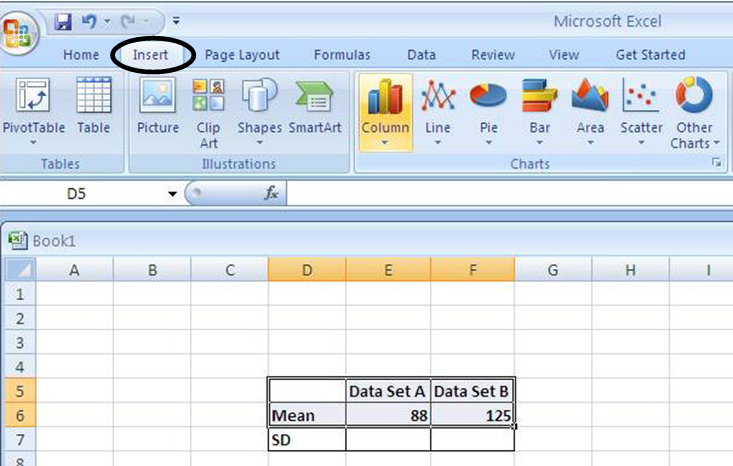
3 Macros to Insert Page Number Using VBA in Excel
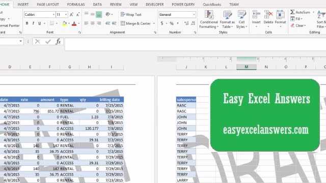
Let’s get introduced to our dataset first that represents some salespersons’ sales in different regions. There are three pages in our sheet.
1. Insert Page Number in Footer Using Excel VBA
In our first macro, we’ll insert the page number in the center of a Footer. So, we’ll have to insert Footer first otherwise this macro won’t work.
Steps:
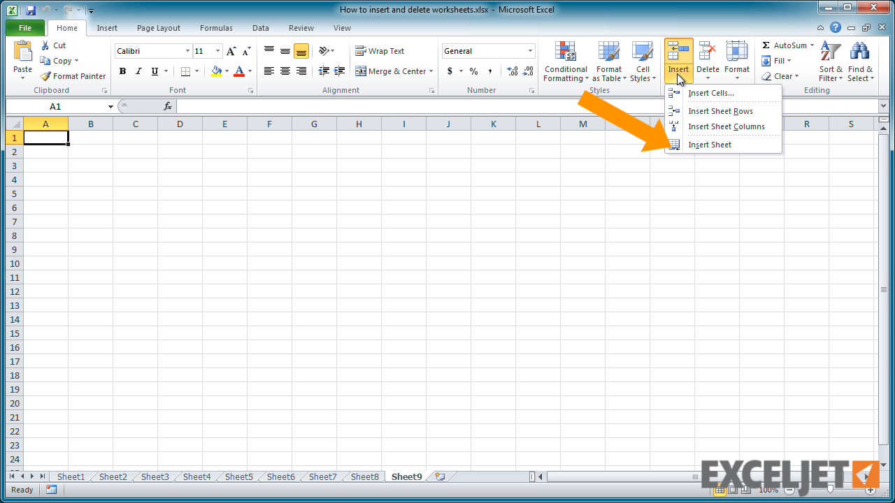
Click as follows to insert a footer: Insert > Text > Header & Footer.
Then scroll down to the page and see that the footer is added.
- Press ALT + F11 to open the VBA
- Then click as follows to insert a new module: Insert > Module.
Later, type the following codes in the module-
After that, go back to your sheet.
Code Breakdown:
- First, I created a Sub procedure- Page_Numbers_inFooter.
- Then declared a variable, Wsheet as Worksheet.
- Later, used the Set and With statement to insert the page number in the center of the footer.
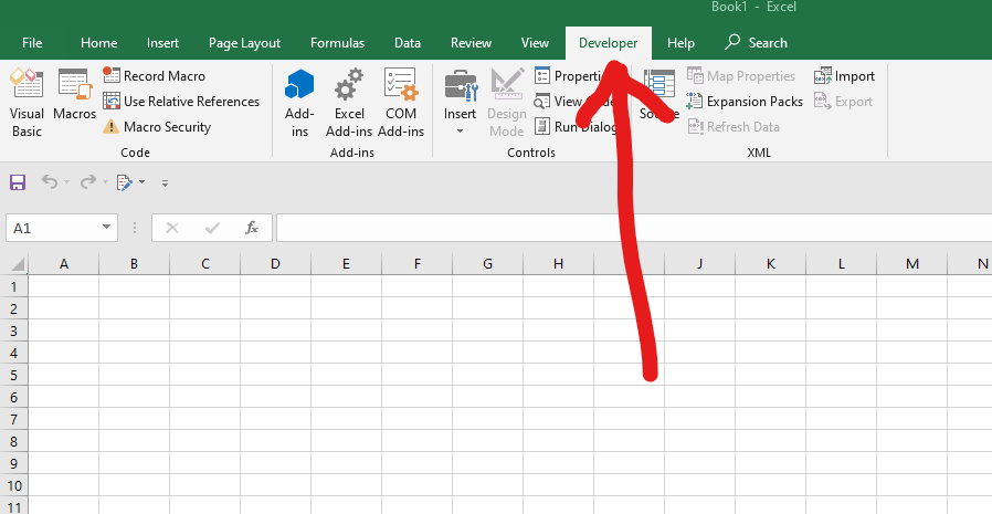
Next, click as follows to open the Macro dialog box: Developer > Macros.
Select the specified Macro name and press Run.
Now see, the macro has inserted the page number in the footer.
2. VBA to Insert Total Page Number in Footer
The previous macro will only insert the page number, and won’t show the page number out of the total number. This macro will show it in the center of the footer of your excel sheet.
Steps:
- Follow the first 3 steps from the first section.
- Then write the following codes in it
Next, go back to your sheet.
Code Breakdown:
- Here, I created a Sub procedure- Total_Page_Number_Footer.
- Then declared a variable, Wsheet as Worksheet.
- Finally, used the Set and With statement to insert the total page number in the center of the footer.
- Follow the 5th step from the first section to open the macro dialog box.
- Select the specified macro name and just press Run.
Now have a look, the page number and the total page number are inserted into the center of the footer.
3. Insert Page Number in Selected Cell
The previous macros would need a footer so we couldn’t insert page numbers in any of our desired locations. By using this macro, we can insert the page number in a specific cell. It will apply the page number in the active sheet. Here well insert the page number in Cell D13.


Steps:
- Follow the first 3 steps from the first section.
- After that, type the following codes in the module-
Later, go back to the sheet.
Code Breakdown:
- First, I created a Sub procedure- Page_Number_Selected_Cell.
- Then declared some variables, mVCount and mHCount As Integer, mVBreak As VPageBreak,mHBreak As HPageBreak, mNumPage As Integer.
- Later, I used If and Else statements to count the page breaks.
- Next, used For loop and If statement to count and increase the page number one by one.
- After that, select the cell where you want to insert the page number.
- Follow the 5th step from the first section to open the Macro dialog box.
- Select the mentioned macro name and finally, just press Run.
Soon after, you will see that the macro has inserted the page number in the specific cell and is showing the total page numbers too.
Worksheet.HPageBreaks property (Excel)
The sheet has a read-only collection called HPageBreaks, which represents the horizontal page breaks.
Syntax
The mentioned text that requires rephrasing is «expression» and «HPageBreaks».
An expression is a variable that represents an object of type Worksheet.
Example
The code snippet provided demonstrates how to show the count of horizontal page breaks in both the full-screen and print-area views.
In the provided code example, a page break is inserted whenever there is a change in the value of a cell within column A.
Support and feedback
If you have any inquiries or suggestions regarding Office VBA or this documentation, please refer to
office vba support
and feedback for assistance on how to receive support and share your feedback.
Excel : how to show page break in normal view by default, Display or hide page breaks in Normal view. Click the File tab > Options. In Excel, click the Microsoft Office Button Office button image , and then click Excel Options. In the Advanced category, under Display options for this worksheet, select or clear the Show page breaks check box to turn page breaks …
Font
Font Name
The value of this property can be set to one of the fonts: Calibri, Times new Roman, Arial…
The following code sets the font name of range A1:A5 to Calibri.
Font Style
The value of this property can be set to one of the constants: Regular, Bold, Italic, Bold Italic.
The following code sets the font style of range A1:A5 to Italic.
Font Size
The value of this property can be set to an integer value from 1 to 409.
The following code sets the font size of cell A1 to 14.
Underline
The value of this property can be set to one of the constants: xlUnderlineStyleNone, xlUnderlineStyleSingle, xlUnderlineStyleDouble, xlUnderlineStyleSingleAccounting, xlUnderlineStyleDoubleAccounting.
The following code sets the font of cell A1 to xlUnderlineStyleDouble (double underline).
Font Color
The value of this property can be set to one of the standard colors: vbBlack, vbRed, vbGreen, vbYellow, vbBlue, vbMagenta, vbCyan, vbWhite or an integer value from 0 to 16,581,375.
To assist you with specifying the color of anything, the VBA is equipped with a function named RGB. Its syntax is:
This function takes three arguments and each must hold a value between 0 and 255. The first argument represents the ratio of red of the color. The second argument represents the green ratio of the color. The last argument represents the blue of the color. After the function has been called, it produces a number whose maximum value can be 255 * 255 * 255 = 16,581,375, which represents a color.
The following code sets the font color of cell A1 to vbBlack (Black).
The following code sets the font color of cell A1 to 0 (Black).
The following code sets the font color of cell A1 to RGB(0, 0, 0) (Black).
True if the font is struck through with a horizontal line.
The following code sets the font of cell A1 to strikethrough.
True if the font is formatted as subscript. False by default.
The following code sets the font of cell A1 to Subscript.
Superscript
True if the font is formatted as superscript; False by default.
The following code sets the font of cell A1 to Superscript.
Page Break along with Subtotal
Now here’s one of the nifty things about Excel; the control over the data. You can have Excel automatically adding page breaks to group categories in a dataset by using the Subtotal feature. Let’s see how to make it happen:


We have sales data regarding a hair salon.
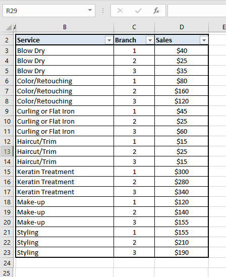
The data can be arranged to group the performance of branches or even the services to highlight which services are the cash cows in the salon. For now, we will check the performance of the branches.
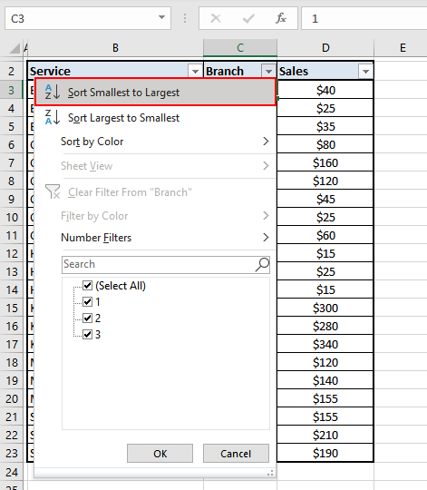
First, we filter the data according to the Branch. Then we apply the Subtotal feature. Find the steps below:
Filter the data, sorting it from smallest to largest.
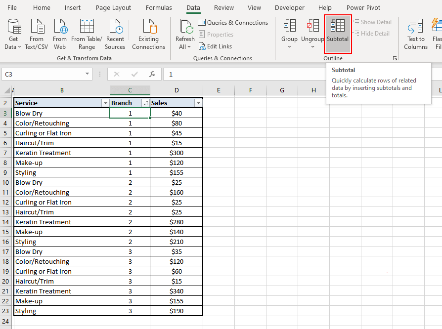
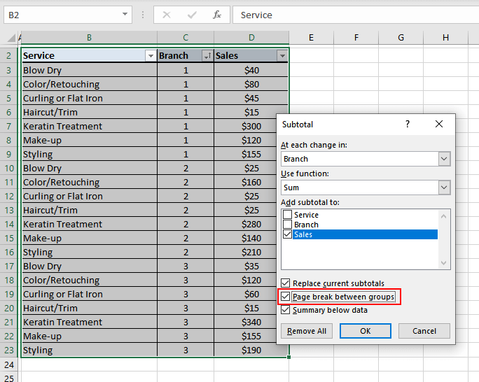
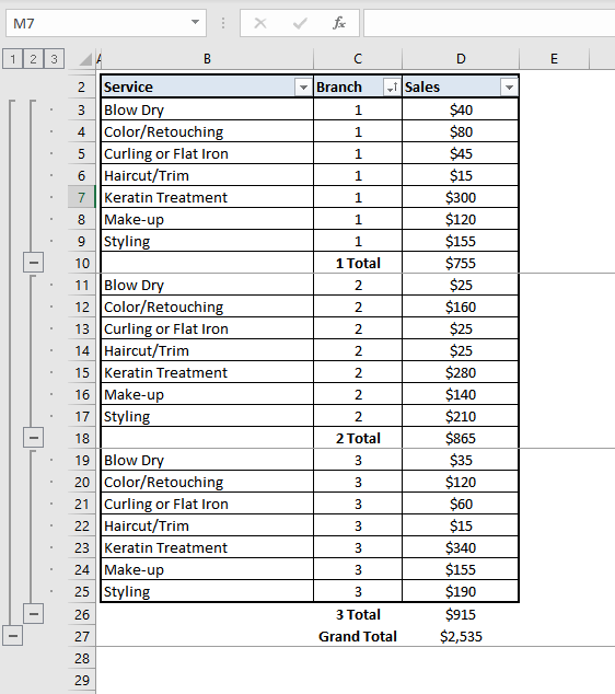
Neat isn’t it? Conveniently, each branch’s data can be printed on separate pages with the totals of each branch and the page breaks added, thanks to the page break option in the Subtotal feature.
We should call the end now. That was really interesting, learning how things can be controlled around the humble page break. Looks like page break got its big break today. Next time you’re having trouble with what to print on your sheets, try taking pointers from this tutorial instead of having a breakdown over page breaks. We always have more from Excel ready for you and we’ll keep it coming.
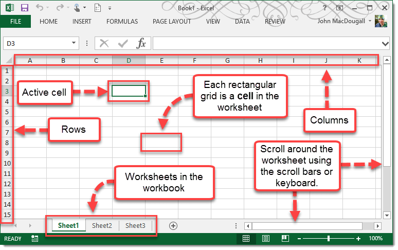
Свойство Range
Рабочий лист имеет свойство Range, которое можно использовать для доступа к ячейкам в VBA. Свойство Range принимает тот же аргумент, что и большинство функций Excel Worksheet, например: «А1», «А3: С6» и т.д.
В следующем примере показано, как поместить значение в ячейку с помощью свойства Range.
Sub ZapisVYacheiku()

    ' Запишите число в ячейку A1 на листе 1 этой книги
    ThisWorkbook.Worksheets("Лист1").Range("A1").Value2 = 67

    ' Напишите текст в ячейку A2 на листе 1 этой рабочей книги
    ThisWorkbook.Worksheets("Лист1").Range("A2").Value2 = "Иван Петров"

    ' Запишите дату в ячейку A3 на листе 1 этой книги
    ThisWorkbook.Worksheets("Лист1").Range("A3").Value2 = #11/21/2019#

End Sub
Как видно из кода, Range является членом Worksheets, которая, в свою очередь, является членом Workbook. Иерархия такая же, как и в Excel, поэтому должно быть легко понять. Чтобы сделать что-то с Range, вы должны сначала указать рабочую книгу и рабочий лист, которому она принадлежит.
В оставшейся части этой статьи я буду использовать для ссылки на лист.
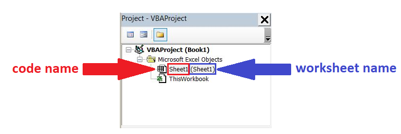
Следующий код показывает приведенный выше пример с использованием кодового имени рабочего листа, т.е. Лист1 вместо ThisWorkbook.Worksheets («Лист1»).
Sub IspKodImya ()

    ' Запишите число в ячейку A1 на листе 1 этой книги
     Sheet1.Range("A1").Value2 = 67

    ' Напишите текст в ячейку A2 на листе 1 этой рабочей книги
    Sheet1.Range("A2").Value2 = "Иван Петров"

    ' Запишите дату в ячейку A3 на листе 1 этой книги
    Sheet1.Range("A3").Value2 = #11/21/2019#

End Sub
Вы также можете писать в несколько ячеек, используя свойство
Range
Sub ZapisNeskol()

    ' Запишите число в диапазон ячеек
    Sheet1.Range("A1:A10").Value2 = 67

    ' Написать текст в несколько диапазонов ячеек
    Sheet1.Range("B2:B5,B7:B9").Value2 = "Иван Петров"

End Sub