
Sleep
Sleep is a Windows API function, that is, it is not part of VBA it is part of the Windows operating system.
But we can access it by using a special declaration statement in our VBA.
This declaration statement serves two purposes. Firstly, it tells Excel where to find the function, secondly it allows us to use the 32bit version of the function in 32bit Excel, and the 64bit version of the function in 64bit Excel.
The Declare statement looks like this
#If VBA7 Then ' Excel 2010 or later

    Public Declare PtrSafe Sub Sleep Lib "kernel32" (ByVal Milliseconds As LongPtr)

#Else ' Excel 2007 or earlier

    Public Declare PtrSafe Sub Sleep Lib "kernel32" (ByVal Milliseconds As Long)

#End If
You can read more about these type of Declare statements and 32bit/64bit Office on Microsoft’s MSDN site
Sleep allows us to pause a macro for X milliseconds, which is a better resolution than Wait which has a minimum delay of 1 second.
So to pause a macro for 5 seconds using Sleep we write this
Sleep 5000
How do I use xlDown in excel VBA?
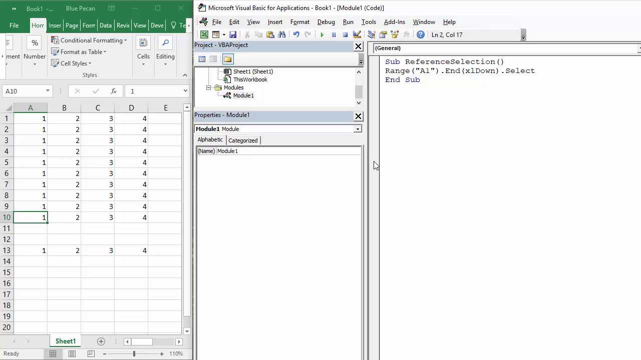
End(xlDown) is the VBA equivalent of clicking Ctrl + Down . This will give you an idea of all the different rows, Ctrl + Down might take you to. Set newRange = ws. Range(“A1”).
What is XLUP and xlDown in VBA?
End(xlUp) vba excel. Assume you have between 25,000 and and 50,000 rows of data in columns 1 to 5,000, every column may have a different number of rows. All data is continuous i.e. there are no empty rows in a column and no empty columns.
What does end XLUP .row do?
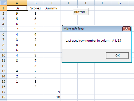
The VBA snippet End(xlup). Row will find the last used row in an Excel range. Knowing the last row in Excel is useful for looping through columns of data.
How do I use xlToRight in VBA?
This example selects the cell at the top of column B in the region that contains cell B4.
- Range(“B4”). End(xlUp). Select.
- Range(“B4”). End(xlToRight). Select.
- Worksheets(“Sheet1”).Activate Range(“B4”, Range(“B4”). End(xlToRight)). Select.
Replace Data Across Multiple Worksheets
Get 30% Discount on Simple Sheets Templates and Courses Use Discount Code BLUE
All enrolments and purchases help this blog(a commission is received at no extra cost to you)
This procedure replaces the name of a store location across specified worksheets in the same workbook.
Sub ReplaceDataAcrossSheets()

Dim ws As Worksheet
'Use the variant data type to store an array of worksheets
Dim Replacews As Variant
'Define the array of worksheets that you want to replace data in
Set Replacews = Worksheets(Array("Replace Sheet1", _
"Replace Sheet2", "Replace Sheet3"))
'replace data with data
For Each ws In Replacews
    ws.UsedRange.Replace What:="Brighton", Replacement:="Bristol"
Next ws

End Sub
The Cells Property of the Worksheet
The worksheet object has another property called Cells which is very similar to range. There are two differences
- Cells returns a range of one cell only.
- Cells takes row and column as arguments.
The example below shows you how to write values to cells using both the Range and Cells property
' https://excelmacromastery.com/
Public Sub UsingCells()

    ' Write to A1
    Sheet1.Range("A1").Value2 = 10
    Sheet1.Cells(1, 1).Value2  = 10

    ' Write to A10
    Sheet1.Range("A10").Value2 = 10
    Sheet1.Cells(10, 1).Value2  = 10

    ' Write to E1
    Sheet1.Range("E1").Value2 = 10
    Sheet1.Cells(1, 5).Value2  = 10

End Sub
You may be wondering when you should use Cells and when you should use Range. Using Range is useful for accessing the same cells each time the Macro runs.
For example, if you were using a Macro to calculate a total and write it to cell A10 every time then Range would be suitable for this task.
Using the Cells property is useful if you are accessing a cell based on a number that may vary. It is easier to explain this with an example.
In the following code, we ask the user to specify the column number. Using Cells gives us the flexibility to use a variable number for the column.
' https://excelmacromastery.com/
Public Sub WriteToColumn()

    Dim UserCol As Integer

    ' Get the column number from the user
    UserCol = Application.InputBox(" Please enter the column...", Type:=1)

    ' Write text to user selected column
    Sheet1.Cells(1, UserCol).Value2 = "John Smith"

End Sub
In the above example, we are using a number for the column rather than a letter.
To use Range here would require us to convert these values to the letter/number cell reference e.g. “C1”. Using the Cells property allows us to provide a row and a column number to access a cell.
Sometimes you may want to return more than one cell using row and column numbers. The next section shows you how to do this.
How to Work with Objects in VBA
After that, the data included in the file that’s located where the FileLocation variable is gets stored into the constant .
Note that we are using the keyword which is mainly used for objects, such as an import of a workbook.
To test whether we are able to extract the date from the file, we again use to print the city, which is located in cell B1 of the files available per the link mentioned in the beginning of this tutorial.
If you import the file , you should see Amsterdam printed in your Immediate Window. After the file is closed, Excel will behave normally again. We can easily paste the (just printed) city name in the in our own template by replacing the with the following:
Note that we can now use our variable to get the data from the imported workbook. But we can also use (protected keyword name by VBA) to get to properties of our own template instead.
If we now run this macro and import , the city should now be printed in the left-upper corner of your Amsterdam worksheet.
Using the Range.Resize Method
When copying from one range to another using assignment(i.e. the equals sign), the destination range must be the same size as the source range.
Using the Resize function allows us to resize a range to a given number of rows and columns.
For example:
' https://excelmacromastery.com/
Sub ResizeExamples()

    ' Prints A1
    Debug.Print Sheet1.Range("A1").Address

    ' Prints A1:A2
    Debug.Print Sheet1.Range("A1").Resize(2, 1).Address

    ' Prints A1:A5
    Debug.Print Sheet1.Range("A1").Resize(5, 1).Address

    ' Prints A1:D1
    Debug.Print Sheet1.Range("A1").Resize(1, 4).Address

    ' Prints A1:C3
    Debug.Print Sheet1.Range("A1").Resize(3, 3).Address

End Sub
When we want to resize our destination range we can simply use the source range size.
In other words, we use the row and column count of the source range as the parameters for resizing:
' https://excelmacromastery.com/
Sub Resize()

    Dim rgSrc As Range, rgDest As Range

    ' Get all the data in the current region
    Set rgSrc = Sheet1.Range("A1").CurrentRegion

      ' Get the range destination
    Set rgDest = Sheet2.Range("A1")
    Set rgDest = rgDest.Resize(rgSrc.Rows.Count, rgSrc.Columns.Count)

    rgDest.Value2 = rgSrc.Value2

End Sub
We can do the resize in one line if we prefer:
' https://excelmacromastery.com/
Sub ResizeOneLine()

    Dim rgSrc As Range

    ' Get all the data in the current region
    Set rgSrc = Sheet1.Range("A1").CurrentRegion

    With rgSrc
        Sheet2.Range("A1").Resize(.Rows.Count, .Columns.Count).Value2 = .Value2
    End With

End Sub
How to Use Arrays in VBA
Every heard of DRY? Don’t Repeat Yourself! Unfortunately, that is exactly what we are doing here.
An alternative could be to store the three headers in an array instead and loop over them to get to the same result. Is that really necessary for three items? Its debatable to be honest. But below you will find my code example as described:
The variant is used as an array, which is declared where you would expect and the titles are inserted later per index direclty after the variable declaration.
Instead of providing the individual cell locations, I have used a loop which runs from zero to the number of items (minus one, as arrays in VBA start at zero too). The title is then printed to the sheet, just like in the previous situation.
You might need to add another header later on, in which case the latest solution is easier. But if you are a hundred percent sure you’ll stick with three only, choose what is most convenient for you. It’s best to know both ways after all.
It does not matter which of the two options you choose for the remainder of this tutorial, as long as you got the headers printed.
Использование VBA в Excel
С помощью VBA вы можете:
- Автоматизировать рутинные задачи: Например, вы можете написать скрипт, который будет автоматически заполнять определенные ячейки данными, выполнять операции с ячейками и т.д.
- Создать пользовательские функции: VBA позволяет создавать свои собственные функции, которые можно использовать в формулах Excel. Таким образом, вы можете добавить свои собственные вычисления или логику в формулы.
- Взаимодействовать с другими программами: С помощью VBA вы можете взаимодействовать с другими программами из пакета Microsoft Office, такими как Word, PowerPoint, Outlook и Access. Вы можете создавать отчеты, отправлять электронные письма и многое другое.
- Настроить пользовательский интерфейс: Вы можете создать пользовательские формы и диалоговые окна, чтобы упростить работу с данными в Excel. Это может быть полезно, если вы хотите, чтобы другие пользователи могли легко взаимодействовать с вашей книгой Excel.
Использование VBA в Excel требует некоторых знаний программирования, но даже базовые навыки в VBA могут существенно упростить вашу работу в Excel. Вы можете начать с создания макросов, которые записывают ваши действия в формате VBA, и затем изменять этот код, чтобы соответствовать вашим потребностям.
Примечание: Для запуска и отладки кода VBA в Excel, вы должны открыть режим разработчика и открыть редактор VBA. Для этого щелкните правой кнопкой мыши на ленте инструментов Excel, выберите «Настроить ленту» и активируйте флажок «Разработка». Затем в разделе «Разработка» выберите «Visual Basic» или используйте горячие клавиши «Alt» + «F11».
About Microsoft Word VBA’s ActiveDocument
The main VBA component that we’ll rely on in both procedures is the ActiveDocument property, which returns a Document object that represents the active document. In other words, this opens the document, as a whole. You won’t need this for every VBA procedure in Word, but you will need it when you need to reference “parts” of the document.
If no Word document is open, this property returns an error. If you’re using this property from inside Excel or PowerPoint, you should include error-handling for this situation.
This property uses the following form:
where is a variable that represents the Application object (Word). Fortunately, in Word, this is implicitly implied.
The next piece of VBA we’ll use is the Range method, which uses the form
to return a Range object. We’ll use this method to identify an area of the document.
There’s no method that says “go to the beginning,” or “go to the end,” so we’ll use the start and end arguments to identify both. Both arguments are optional, and as you might suspect, identifies the first character position and identifies the last character position.
Now, let’s move on to the actual VBA procedures.
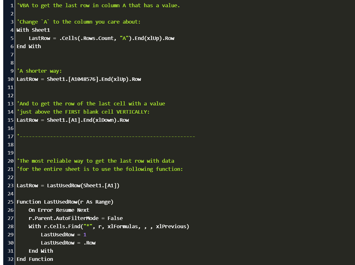
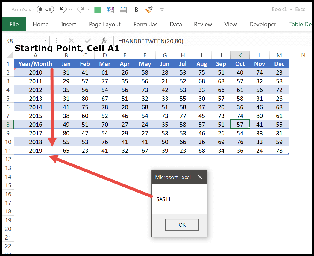
Определение последней ячейки в диапазоне с помощью VBA Excel
Для работы с ячейками в VBA Excel необходимо знать конечную ячейку диапазона. Это может быть полезно, например, для управления циклами или для проверки, что все данные были обработаны. В VBA существует несколько способов определить последнюю ячейку в диапазоне, включая использование метода End, поиска пустых ячеек или специальных функций.
Один из способов определения последней ячейки в диапазоне — использование метода End. Метод End может быть применен к объекту Range и позволяет определить последнюю ячейку в диапазоне в указанном направлении (вниз, вправо, вверх или влево).
Например, следующий код определяет последнюю заполненную ячейку в диапазоне A1:B10:
В данном примере, метод End(xlDown) определяет последнюю заполненную ячейку вниз от ячейки A1 в диапазоне A1:B10. Результатом будет ячейка, которая является последней по вертикали в этом диапазоне.
Если вам нужно определить последнюю заполненную ячейку в горизонтальном направлении, вы можете использовать метод End(xlToRight). Например:
В данном примере, метод End(xlToRight) определяет последнюю заполненную ячейку вправо от ячейки A1 в диапазоне A1:B10. Результатом будет ячейка, которая является последней по горизонтали в этом диапазоне.
Также можно определить последнюю заполненную ячейку в диапазоне с помощью функций, таких как Find и SpecialCells. Например:
В данном примере, метод Find ищет последнюю заполненную ячейку в диапазоне A1:B10, используя астриск (*) в качестве критерия поиска. Результатом будет ячейка, которая является последней заполненной ячейкой в диапазоне.
Это лишь некоторые из способов определить последнюю ячейку в диапазоне с помощью VBA Excel. Вы можете выбрать тот, который наилучшим образом подходит для вашей ситуации.
Расширение возможностей Excel с помощью VBA
Microsoft Excel – это одна из самых популярных программ для работы с электронными таблицами. Она предоставляет множество функций и возможностей для обработки и анализа данных. VBA (Visual Basic for Applications) – это язык программирования, который позволяет дополнить Excel дополнительными функциональными возможностями.
С использованием VBA можно создавать макросы, автоматизировать рутинные задачи, анализировать данные, генерировать отчеты и многое другое. При помощи VBA можно обращаться к ячейкам, столбцам и строкам таблицы, изменять их значения, форматирование, создавать новые листы и книги Excel.
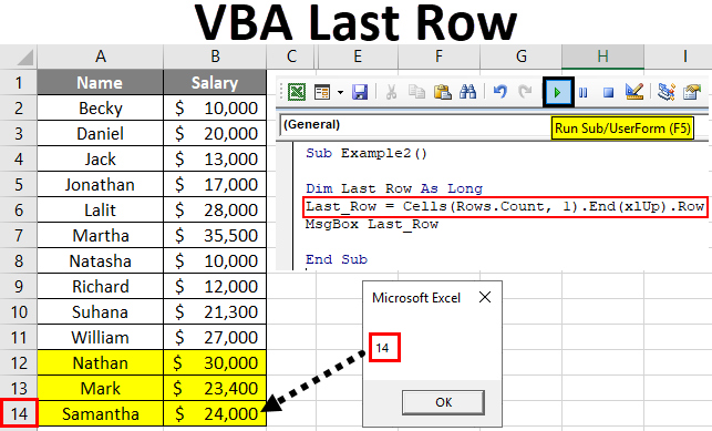
Одной из наиболее полезных функций VBA является возможность найти последнюю заполненную ячейку в таблице. На практике это может быть очень полезно, например, для поиска последней строки с данными или для определения диапазона данных, который нужно обработать.
Для поиска последней заполненной ячейки в Excel VBA можно использовать несколько способов:
- Использование свойства «End». Этот способ позволяет найти последнюю заполненную ячейку в определенном столбце или строке. Например:
| Код | Описание |
|---|---|
| lastRow = Cells(Rows.Count, «A»).End(xlUp).Row | Поиск последней заполненной ячейки в столбце «А» |
| lastColumn = Cells(1, Columns.Count).End(xlToLeft).Column | Поиск последней заполненной ячейки в первой строке |
Использование функции «Find». Этот способ позволяет найти конкретное значение в таблице и вернуть адрес этой ячейки. Например:
| Код | Описание |
|---|---|
| Set rng = Range(«A1:Z100»).Find(«Value») | Поиск ячейки со значением «Value» в диапазоне «A1:Z100» |
Использование функции «CurrentRegion». Этот способ позволяет определить диапазон данных вокруг конкретной ячейки. Например:
| Код | Описание |
|---|---|
| Set rng = Range(«A1»).CurrentRegion | Определение диапазона данных вокруг ячейки «A1» |
VBA обладает мощными возможностями для автоматизации работы с Excel. Он позволяет создавать пользовательские функции, взаимодействовать с другими приложениями Microsoft Office, выполнять сложные математические и статистические расчеты, а также создавать пользовательские интерфейсы для взаимодействия с данными.
Если вы хотите расширить возможности Excel и сделать свою работу более эффективной, рекомендуется изучить VBA. С его помощью вы сможете автоматизировать повторяющиеся действия, провести сложные анализы данных и создать удобные пользовательские интерфейсы.
How to Build a Macro with Visual Basic for Applications
Now that we have set the parameters, we can move on with actually building the macro.
If this is the first time you are using VBA, you might need to customize your ribbon to get the necessary functions available.
In order to do so, make sure that the Developer box is ticked (as shown in Figure 3 below) and that the Developer options are available in your ribbon after you have saved your changes.
 Figure 03: Settings Excel
You should now be able to open Visual Basic from the Developer tab in Excel, which should look something like this:
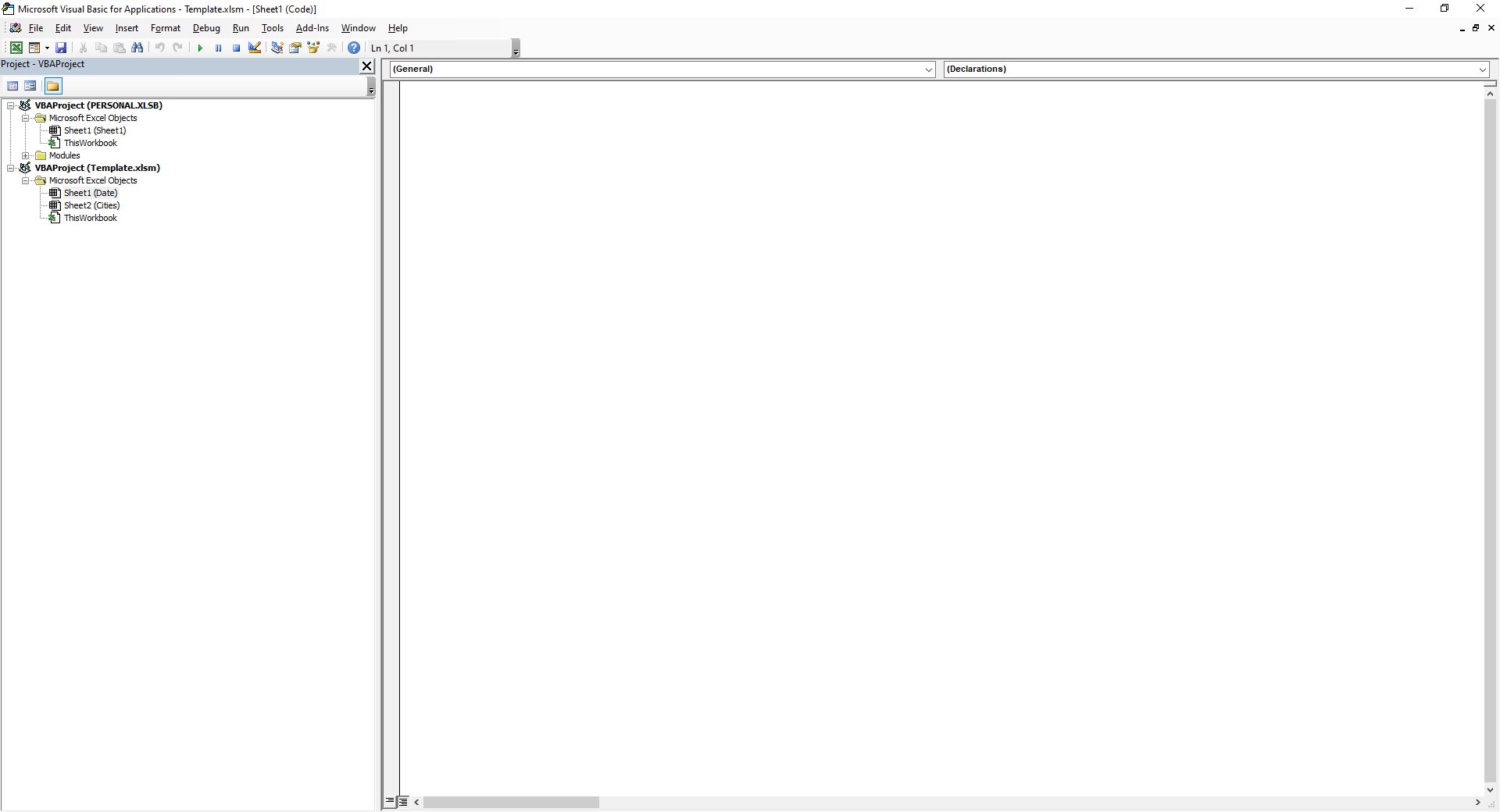 Figure 04: Visual Basic
This is the editor provided by Excel where you will be able to create, adjust, and remove your functions and macros. I will not go into too much detail for now, but I’ll just explain some of the elements as we go.
Now, let’s got our hands dirty and write our first macro. You could choose to write macros for a single worksheet only, or choose to have them available in the entire workbook.
As the two worksheets we created earlier only maintain the parameters, I chose to write the macros for the entire workbook by double-clicking the «ThisWorkbook» option in the sidebar for our project.
Don’t worry about the PERSONAL.xlsb in my screenshot for now – this is a file containing functions that I can use in all my files and will be handled in a future tutorial.
How to Create Our First Macro
After you’ve selected the workbook, you are ready to start your first program.
Macros in VBA start with the keyword Sub, short for subroutine, followed by their name and two parentheses. Although the editor is nothing compared to an IDE like Visual Studio Code, it will complete the code with End Sub when you hit enter after the two parentheses.
For now, I have created an empty macro called which looks like this:
It is a bit sad that the function does not do anything for now, so let’s add the following code and find out what it does:
If we were to run this code right now, the function would create a new worksheet in our Excel workbook called NewSheet.
Note that I have included a comment in the code by starting the line with an apostrophe. This will not be executed, but is only there to help you and myself understand the code.
We can run this code by placing our cursor somewhere in the function and pressing the green ‘play’ icon on top of the editor, which says Run Sub when you hover over it.
After you have pressed this button, you will see that new worksheet called NewSheet has been created in our workbook and has also been added in the sidebar, next to the sheets we already had.
Personally, I do not like the fact that the sheet is created next to the sheet we had (maybe on purpose, maybe not) selected. Therefore, I will add a parameter to the add method to define its location:
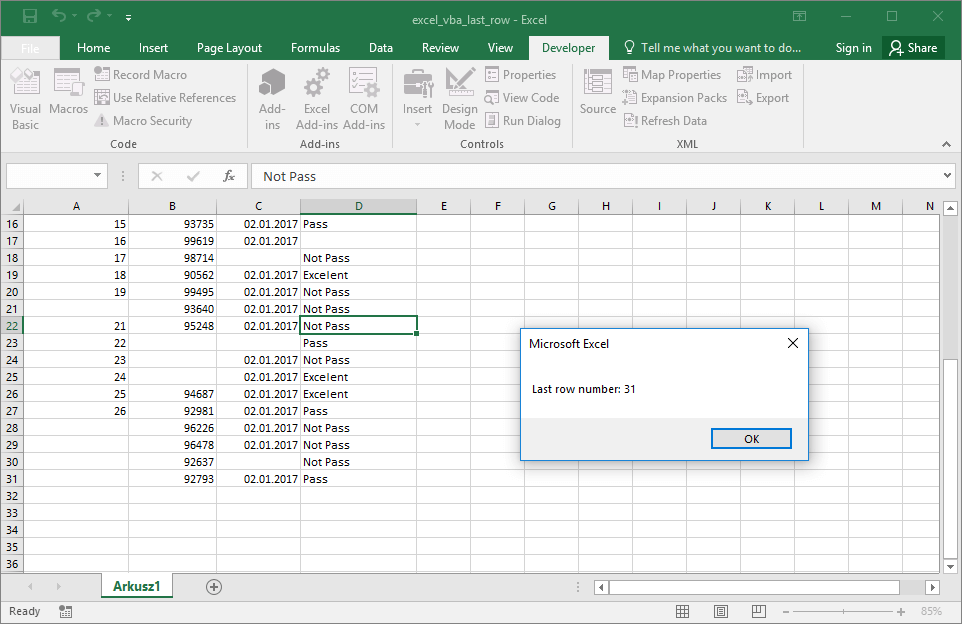
Delete the newly created sheet, as we will now create the worksheets for every city we defined earlier. As the number of cities entered might differ, we want to know how many rows are actually being used in our Cities worksheet.
To test whether we are able to extract the date from the file, we use (similar to print in Python or console.log in JavaScript) to print the numbers of rows, which Excel will calculate for us based on the code we provided.
Make sure to open your Immediate Window (in Visual Basic, by selecting View > Immediate Window) and run the macro above. It will print six, just like we expect, after we have defined the same number of cities in our Cities worksheet earlier in this tutorial.
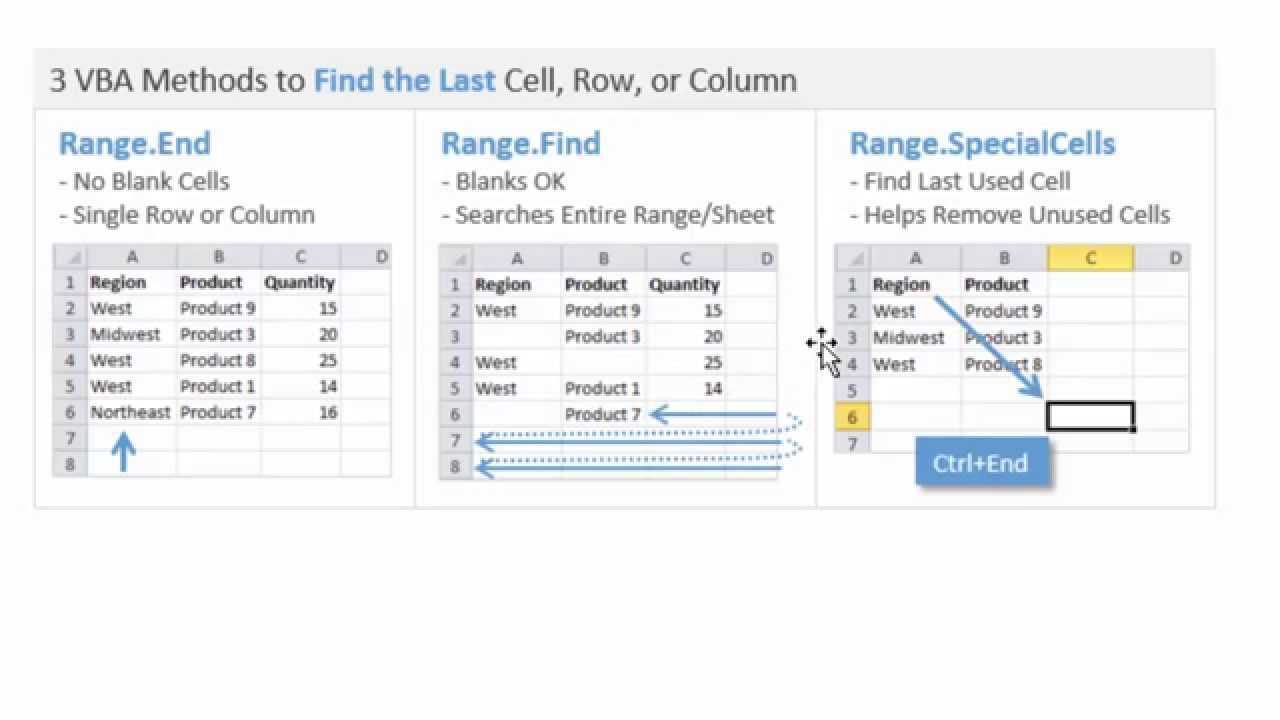
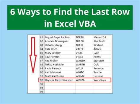
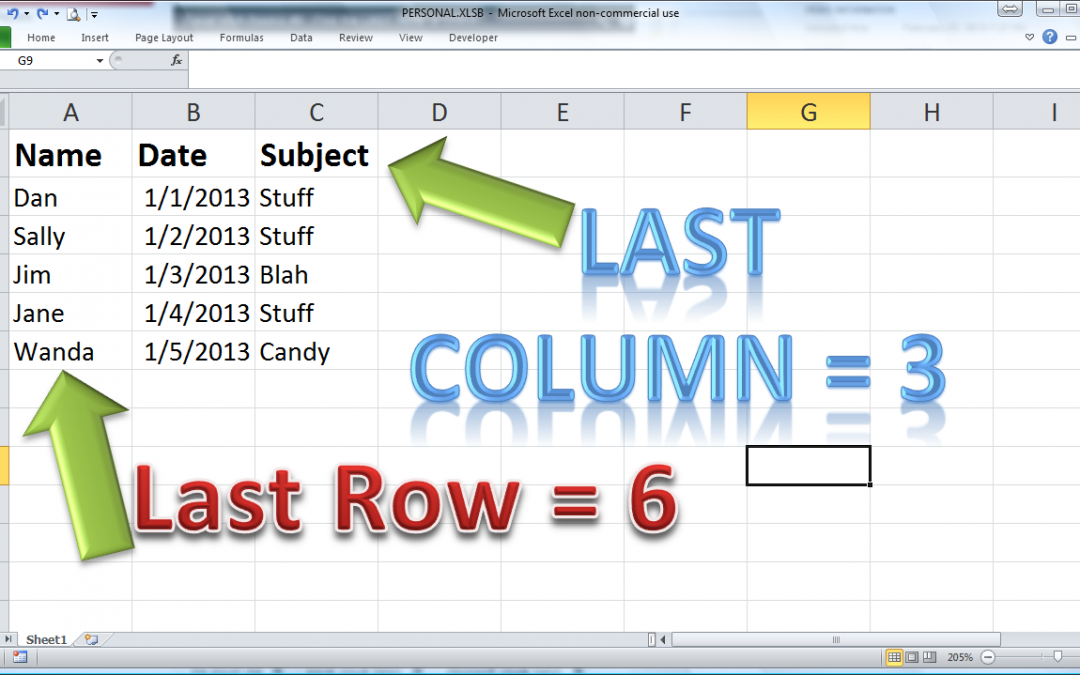
VBA Strategies
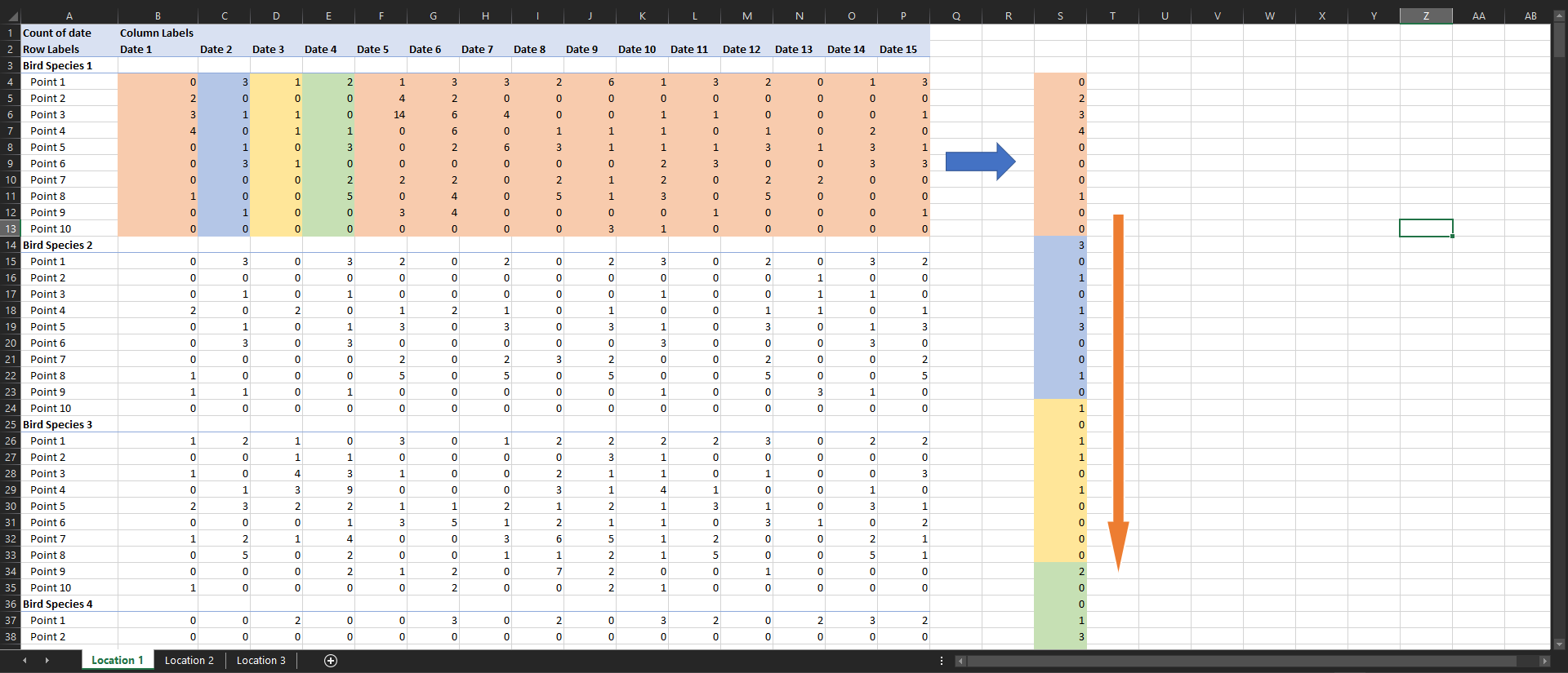
I will look at some of the available strategies for finding the last row.
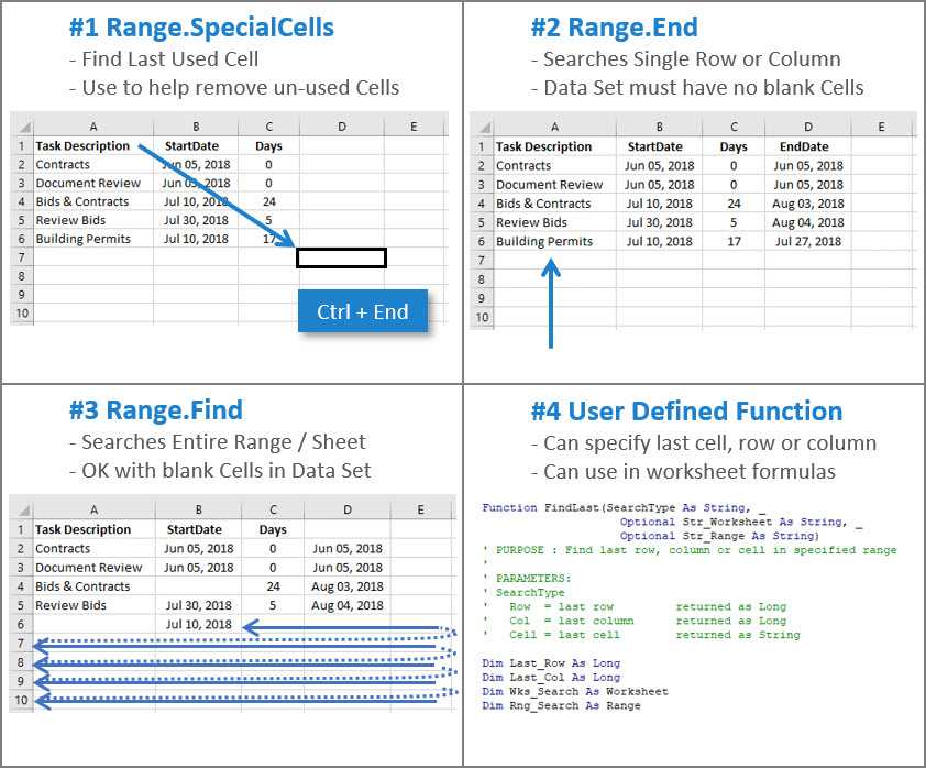
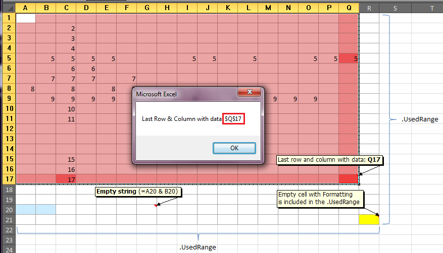
Used Range
Because Excel internally uses a sparse matrix scheme for the cells in each worksheet (instead of holding a gigantic 16384 by 1048576 array) it has to store information for each cell that has been used. So formatted cells are considered used, as well as cells containing values and formulas. Cells remain flagged as used even when all formatting, values and formulas are removed.
Two VBA methods for working with the used range are Worksheet.UsedRange and the xlCellTypeLastCell option of SpecialCells.
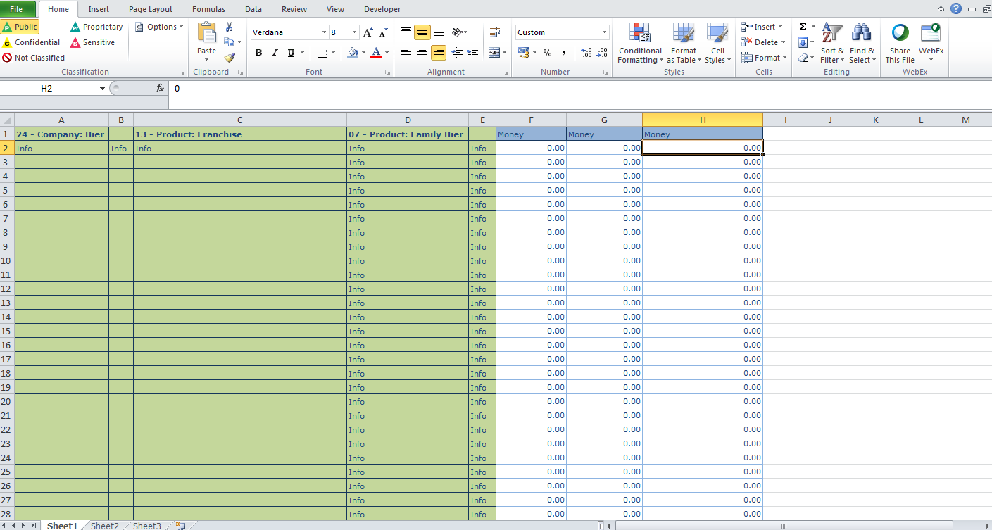

'
' last row in used range
'
jLastUsed = oSht.UsedRange.Rows(oSht.UsedRange.Rows.Count).Row
'
' last visible row in used range
'
jLastVisibleUsed = oSht.Cells.SpecialCells(xlCellTypeLastCell).Row
For my test data jLastUsed returns 42 because there is some formatting on that row, and xlCellTypeLastCell returns 39, which is the last visible row before row 42.
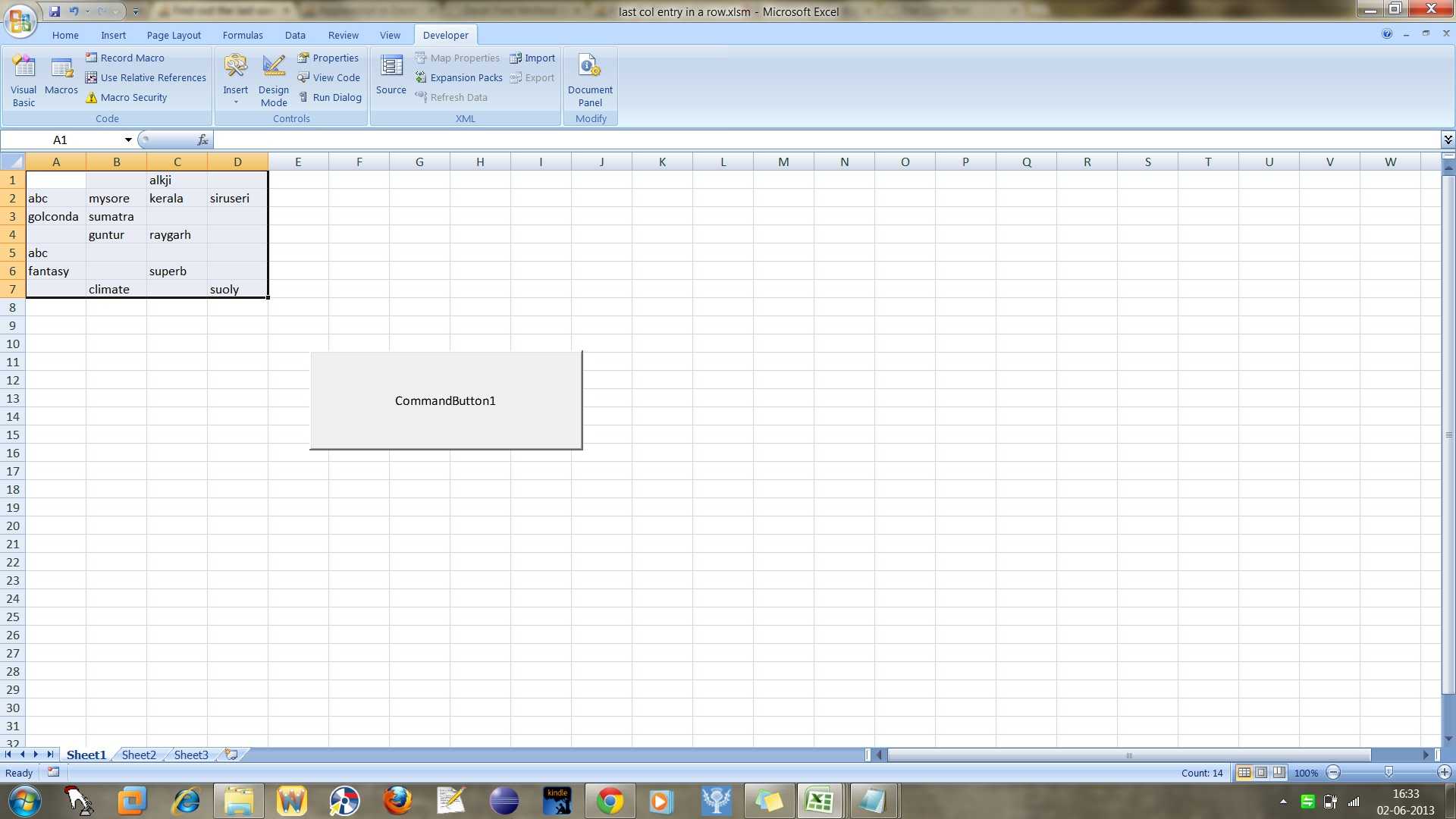
Range.End(xlDown) and Range.End(xlUp)
These VBA methods mimic pressing Ctrl and the up and down arrows.
For name ranges they skip hidden rows but stop at the row before an empty cell.:
'
' last visible cell in Named Range using End(xlUp)
'
jLastVisibleRange = oSht.Range("NamedRange").Offset(oSht.Range("NamedRange").Rows.Count, 0).End(xlUp).Row
'
' last visible cell in Named Range using End(xlDown)
'
jLastVisibleRange2 = oSht.Range("NamedRange").End(xlDown).Row
When using End(xlUp) you want start outside the range in an empty cell, so I used Offset to get to the first row below the range. jLastVisibleRange returns 20.
Using End(xlDown) is simpler for a Range: the code start at the first row in the range and ends at the first of the last visible row in the range that contains data and the last row before an empty cell. It also returns 20.
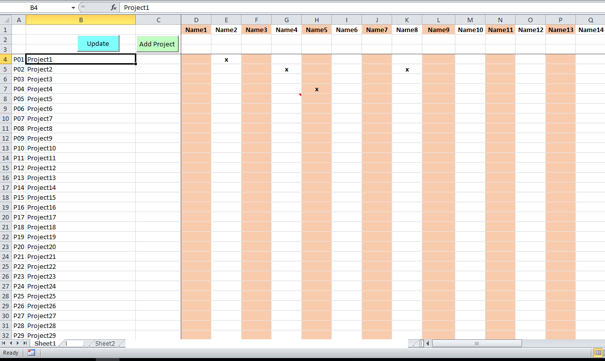
But for Tables End(xlUp) does NOT skip hidden rows!
'
' last row in Table using End(xlUP) - Note End(xlUp ) behaves differently for tables - includes hidden rows
'
jLastInTable2 = oSht.Range("Table1").Offset(oSht.Range("Table1").Rows.Count + 1, 0).End(xlUp).Row
'
' last visible table row using End(xlDown)
'
jLastVisibleTable = oSht.Range("Table1").End(xlDown).Row
So using End(xlUp) starting from the first row after the end of the table returns Row 25 even though that row is hidden.
But End(xlDown) works the same way with a table as with a Range, and so returns row row 20 which is indeed the last visible row in the table.
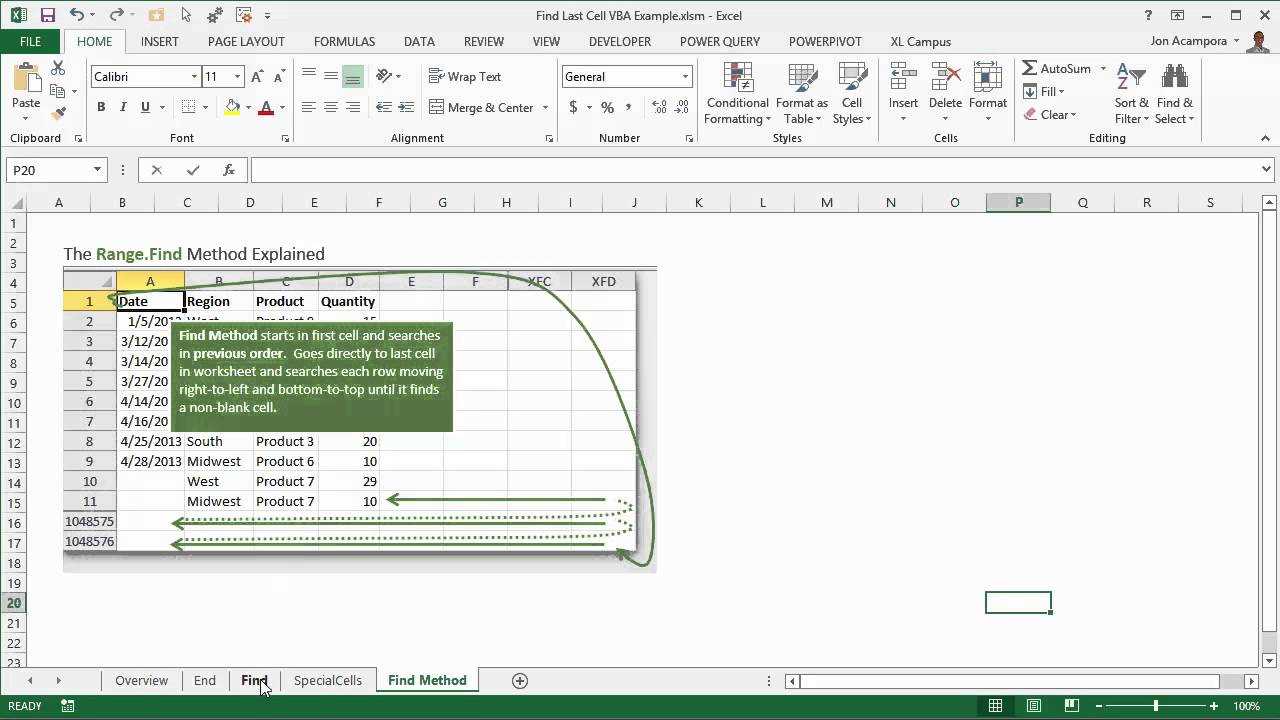
Range.Find
My favourite method is to use Range.Find.
Using Find on Formulas includes hidden rows, whereas using Find on Values excludes hidden rows.
You can use this method on Worksheet.Cells or on a Range or Table.
'
' last row containing data (using Find in formulas)
'
jLastRangeData = oSht.Range("NamedRange").Find(What:="*", LookIn:=xlFormulas, SearchOrder:=xlByRows, SearchDirection:=xlPrevious).Row
'
' last visible row containing data (using Find in values)
'
jLastVisibleRangeData = oSht.Range("NamedRange").Find(What:="*", LookIn:=xlValues, SearchOrder:=xlByRows, SearchDirection:=xlPrevious).Row
'
' last row containing data (using Find in formulas)
'
jLastTableData = oSht.ListObjects("Table1").Range.Find(What:="*", LookIn:=xlFormulas, SearchOrder:=xlByRows, SearchDirection:=xlPrevious).Row
'
' last visible row containing data (using Find in values)
'
jLastVisibleTableData = oSht.ListObjects("Table1").Range.Find(What:="*", LookIn:=xlValues, SearchOrder:=xlByRows, SearchDirection:=xlPrevious).Row
- jLastRangeData returns 25
- jLastVisibleRangeData returns 20
- jLastTableData returns 25
- jLastVisibleTableData returns 20
Methods using COUNT
Sometimes its simpler to just count the number of rows, add the starting row number and subtract 1.
‘
‘ last cell in Named Range
‘
jLastInRange = oSht.Range(«NamedRange»).Offset(oSht.Range(«NamedRange»).Rows.Count – 1, 0).Row
‘
‘ last row in named range current region
‘
jLastInRegion = oSht.Range(«NamedRange»).CurrentRegion.Rows.Count + oSht.Range(«NamedRange»).Row – 1
‘
‘ last row in Table
‘
jLastInTable = oSht.ListObjects(«Table1»).Range.Rows.Count + oSht.ListObjects(«Table1»).Range.Row – 1
‘
‘ last data row in table (excludes total row)
‘
jLastTableDataRow = oSht.ListObjects(«Table1»).ListRows.Count + oSht.ListObjects(«Table1»).Range.Row – 1
- jLastInRange returns 30 (it counts the empty cells too)
- jLastInRegion returns 25 (it excludes the bounding empty cells)
- jLastInTable returns 25
- jLastTableDataRow returns 24 (ListObject.ListRows excludes the total row and header row so I have not subtracted 1 for the header row)
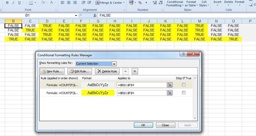
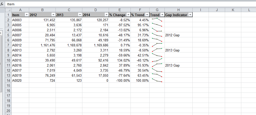
Format Cells Based on Data Type
This procedure formats cells based on data type – number, text, error, logical etc.
Sub FormatCellsBasedonDataType()
Dim rg As Range
Dim list As Range
Set list = Range("A1:A8")

For Each rg In list
    Select Case True
        Case Is = WorksheetFunction.IsError(rg)
        rg.Interior.Color = vbCyan
        Case Is = IsEmpty(rg)
        rg.Interior.Color = vbBlack
        Case Is = WorksheetFunction.IsFormula(rg)
        rg.Interior.Color = vbRed
        rg.Font.Color = vbWhite
        Case Is = WorksheetFunction.IsText(rg)
        rg.Interior.Color = vbGreen
        Case Is = WorksheetFunction.IsNumber(rg)
        rg.Interior.Color = vbYellow
        Case Is = WorksheetFunction.IsLogical(rg)
        rg.Interior.Color = vbBlue
        rg.Font.Color = vbWhite
    End Select
Next rg

End Sub
The code above relates to the data displayed below.
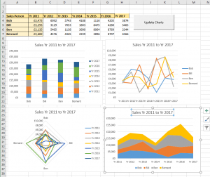
Charts
Get 30% Discount on Simple Sheets Templates and Courses Use Discount Code BLUE
All enrolments and purchases help this blog(a commission is received at no extra cost to you)
This procedure loops through the collection of the chart objects on Sheet1 and adds a title to each chart.
Sub TitleCharts()
Dim AChart As ChartObject
Dim LastYear As String
Dim FirstYear As String
Dim ChartData As Range
Set ChartData = Range("A3").CurrentRegion

For Each AChart In Sheet1.ChartObjects
    FirstYear = Range("a3").Offset(0, 1).Value
    LastYear = Range("a3").End(xlToRight).Value
    With AChart.Chart
        .SetSourceData ChartData
        .HasTitle = True
        .ChartTitle.Select
        .ChartTitle.Text = "Sales " & FirstYear & " to " & LastYear
        .HasLegend = True
    End With
Next

End Sub
The code above relates to the data shown below.
Nested For Each Next
This procedure formats cells based on data type on all sheets in the current workbook. It uses two For Each Next loops. The first For Each Next loop loops through all worksheets in the current workbook. The second For Each Next loop is nested in the first and loops through each cell in the used part of the worksheet.
Sub FormatCellsBasedonDataTypeAcrossWorkbooks()
Dim rg As Range
Dim ws As Worksheet

For Each ws In ThisWorkbook.Worksheets
    For Each rg In ws.UsedRange
        Select Case True
            Case Is = WorksheetFunction.IsError(rg)
            rg.Interior.Color = vbCyan
            Case Is = IsEmpty(rg)
            rg.Interior.Color = vbBlack
            Case Is = WorksheetFunction.IsFormula(rg)
            rg.Interior.Color = vbRed
            rg.Font.Color = vbWhite
            Case Is = WorksheetFunction.IsText(rg)
            rg.Interior.Color = vbGreen
            Case Is = WorksheetFunction.IsNumber(rg)
            rg.Interior.Color = vbYellow
            Case Is = WorksheetFunction.IsLogical(rg)
            rg.Interior.Color = vbBlue
            rg.Font.Color = vbWhite
        End Select
    Next rg
Next ws

End Sub